Software Diagnostics Library

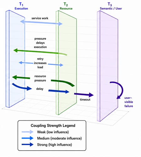
The Trace Multiphysics analysis pattern applies several Trace Fields to the same sequence of trace messages and studies both their individual strengths and their interactions. A Trace Field associates every message in a trace domain M with a value in some analytical range T. Although the field is defined over M, its values need not be extracted solely from that trace. A value may be derived from the message itself, inferred from its surrounding context, or assigned using correlated evidence from other traces, logs, metrics, memory dumps, snapshots, models, or external knowledge sources. The value does not need to be numerical, although numerical or ordered values are useful when field strength must be visualized. For example, one field may represent execution significance, another resource pressure, and a third semantic or user-visible importance:

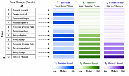
However, Trace Multiphysics is not merely the display of several independent Trace Fields: its essential feature is their coupling. A change in one field may affect another field. For example, increased resource pressure may slow execution. Slower execution may trigger retries. Repeated retries may further increase resource pressure. Eventually, the combined effect may change the semantic or user-visible outcome. The coupling diagram represents these relationships, and arrow thickness indicates coupling strength:

A simple conceptual form is: C_ij​(m)=g(f_i​(m), f_j​(m), R_ij​(m)), where f_i​: M → T_i and f_j​: M → T_j, f_i(m) and f_j(m) are the strengths or values of fields i and j at message m, C_ij(m) is the coupling between fields i and j at message m, and R_ij(m) represents evidence of an interaction between the two fields, obtained from the trace itself or from correlated diagnostic sources. This formula defines coupling at message m. More generally, a coupling may relate field values at different messages when the influence is delayed or propagated through the trace: C_ij​(m_a, m_b)=g(f_i​(m_a), f_j​(m_b), R_ij​(m_a, m_b)), where m_a ⪯ m_b. Here, R_ij​(m_a, m_b) represents evidence relating the value f_i(m_a) of field i to the value f_j(m_b) of field j, whether that evidence is contained in the primary trace or supplied through correlated artifacts. High values in two fields do not automatically establish strong coupling. The available diagnostic evidence must also support the conclusion that one field influences, constrains, amplifies, transforms, or explains the other. Such evidence may occur in the primary trace or in correlated traces, logs, metrics, snapshots, models, or other diagnostic artifacts:

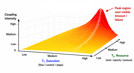
The mapping f_i is defined over the trace domain M, but its construction may depend on evidence outside M. A more explicit form is: f_i(m) = h_i(m, E_i(m)), where E_i(m) is the evidence associated with message m. This evidence may come from the message itself, nearby messages, other traces or logs, metrics, snapshots, memory dumps, learned models, or other correlated diagnostic sources. Correlation may be established through timestamps, identifiers, causal links, shared entities, execution context, or other relations.

When no ordinary field value can be assigned, T_i may include special values representing unknown, unavailable, or not applicable, preserving the definition of the field over the complete trace domain.

In computational modeling, multiphysics simulation studies several aspects of a physical system and their interactions simultaneously. A model may combine thermal, structural, fluid, electromagnetic, or other processes, together with the coupling and boundary conditions between them. Trace Multiphysics transfers this structural principle to software diagnostics. The analogy does not imply that all software behavior should be described by physical equations. Instead, it provides a disciplined way to analyze several interacting dimensions without reducing the incident to one isolated perspective.

The connection is especially appropriate in software diagnostics because software can be its own model. Software execution states and execution artifacts can be copied, preserved, replayed, or analyzed independently. Traces, logs, metrics, memory dumps, and snapshots are symbolic and digital artifacts produced by the software system itself. In this diagnostic sense, software performs a form of self-simulation: its execution generates artifacts that model selected aspects of its own structure and behavior. A trace is not a complete reproduction of the running system. It is a selective, instrumented self-model. Different Trace Fields map messages in that self-model to values in different analytical ranges, each representing a distinct analytical dimension. Some values may be extracted directly from the trace, while others may be inferred, enriched, or projected from correlated traces, logs, metrics, memory dumps, snapshots, models, or external knowledge. Trace Multiphysics studies those fields together and examines how they interact. Thus, multiphysics simulation models several interacting physical processes, whereas Trace Multiphysics analyzes several interacting fields defined over a software-generated model of software behavior and potentially enriched from other diagnostic sources.

Trace Field provides the foundational assignment or mapping from trace messages to values in one analytical range. The field is defined over a selected trace domain, but the evidence used to assign its values may originate inside or outside that domain. Trace Multiphysics extends this principle by applying several Trace Fields to the same trace domain and analyzing their simultaneous values, changing strengths, overlap at individual messages, dependencies, feedback loops, coupling strengths, and combined explanatory effects. The relationship can be summarized as follows: Trace Field maps trace messages to values in one analytical range, while Trace Multiphysics studies several coupled Trace Fields defined over the same trace domain, with their values potentially derived from or enriched by evidence from multiple diagnostic sources.

Trace Multiphysics also connects to several recent analysis patterns. In Trace Reactance, inductive and capacitive effects can be understood as specific forms of inter-field coupling and temporal distortion produced by interacting state fields. Karnaugh Map is also multidimensional but primarily Boolean and combinatorial, whereas Trace Multiphysics accommodates continuous or graded fields, propagation, and feedback loops. Trace World may provide a broader shared diagnostic context in which coupled Trace Fields are interpreted. Bethe Ansatz is a constrained form of Trace Multiphysics in which global behavior is reconstructed from composable pairwise interaction motives.

The pattern is particularly relevant to AI/ML and agentic AI systems. Multiphysics approaches in machine learning usually apply ML to coupled physical processes or incorporate multiple physical priors into learning. Multiphysics-Inspired AI/ML Observability and Diagnostics, by contrast, treats the AI/ML system itself as a collection of interacting analytical fields, including data, optimization, information, computation, uncertainty, control, and semantic outcome fields, defined over a common trace domain constructed from correlated training, inference, and operational events. Its observability aspect concerns the instrumentation, correlation, and enrichment required to construct these fields from training logs, model evaluations, infrastructure metrics, distributed traces, tool-call records, user interactions, safety assessments, and other evidence sources. Its diagnostic aspect concerns how fields interact through their values and couplings, how disturbances propagate across fields, how feedback loops emerge among them, and how their combined effects produce system-level behavior.

In an agentic AI system, for example, increased tool latency may cause retries. Retries may enlarge the accumulated context and increase computational pressure. Context growth may change the relative prominence of relevant information and increase uncertainty, affecting planning, tool selection, and the final semantic outcome. A degraded outcome may provoke further retries, creating a reinforcing feedback loop. Observability provides the correlated evidence needed to construct, expose, and track these fields, while diagnostics analyzes their values and couplings to explain the resulting agent behavior. The behavior cannot be explained adequately by any one field in isolation.

In summary, Trace Multiphysics is a trace and log analysis pattern that examines several Trace Fields defined over the same trace domain, whether their values are derived from that trace alone or assigned using correlated evidence from other diagnostic sources. It studies the immediate, delayed, reinforcing, constraining, transforming, and explanatory couplings through which their combined behavior emerges. Multiphysics-Inspired AI/ML Observability and Diagnostics extends this principle to AI/ML and agentic systems: observability constructs and exposes the relevant fields from distributed evidence, while diagnostics analyzes their interactions and explains the emergent system behavior.

- Dmitry Vostokov @ DumpAnalysis.org + TraceAnalysis.org -

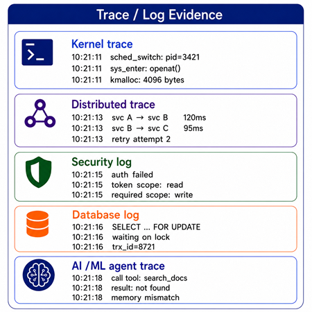
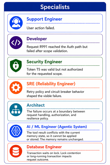
Even when all relevant events are present in traces and logs, they may still remain opaque because the analyst lacks the specialized skill needed to interpret their messages, abstractions, timing, domain vocabulary, failure semantics, or their role in the broader Trace World:

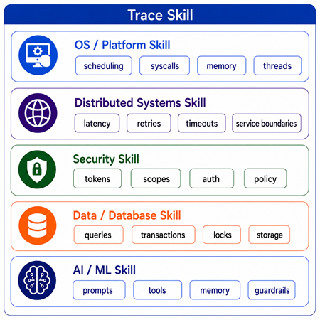
Trace Skill is a trace and log analysis pattern in which successful interpretation depends on a specific skill set required by the trace domain or Trace Ontology:

Some traces can be read with general diagnostic experience, especially if domain-independent analysis patterns are used. Others require specialist knowledge:

• Kernel tracing requires OS internals skill.
• Distributed traces require distributed systems skill.
• Database logs require query, transaction, and storage skill.
• Security logs require identity, policy, token, and threat-modeling skill.
• ML/AI traces require model, prompt, embedding, evaluation, and agentic workflow skill.
• Performance traces require latency, contention, scheduling, and resource-analysis skill.
• Business-process traces require domain workflow knowledge.

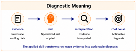
The same trace may therefore be simple for one analyst and almost invisible for another. Even the same analysis pattern may be applied differently. The problem is not the absence of data but the absence of the interpretive skill needed to turn trace data into diagnostic meaning:

Trace Skill analysis pattern may be useful in the following situations:

• The trace contains relevant evidence, but the analyst does not recognize it.
• Messages are dismissed as noise because their domain meaning is unknown.
• A team reads only the parts of the trace matching its own expertise.
• Different specialists disagree because each understands only one layer.
• The trace crosses technical boundaries: application, infrastructure, security, data, ML, business logic.
• The incident is repeatedly escalated because no one possesses the required combination of skills.

Compared to other analysis patterns, Trace Viewpoints are perspectives from which the trace is read. Trace Skill is the competence needed to read from a viewpoint correctly. So a viewpoint can be chosen quickly, but a skill has to be possessed, acquired, or borrowed from someone else. Trace World allows movement across skill sets by creating a common diagnostic language, but Trace Skill explains why this is necessary: traces are often multi-skill artifacts. No single narrow skill may be enough. The analyst either needs multiple skills or needs to collaborate across skill boundaries using a shared Trace World.

We can also say that Trace Skill is needed to navigate traces and logs and their Trace World. Trace World provides the shared diagnostic terrain constructed from trace and log evidence, entities, relations, events, timelines, and viewpoints. Trace Skill is the specialized competence required to navigate both the raw evidence and the reconstructed world accurately, recognize relevant signals, switch between viewpoints, and avoid misinterpretation.

In summary, Trace Skill is a trace and log analysis pattern in which decisive diagnostic evidence can only be recognized by the appropriate specialist skill set.

- Dmitry Vostokov @ DumpAnalysis.org + TraceAnalysis.org -

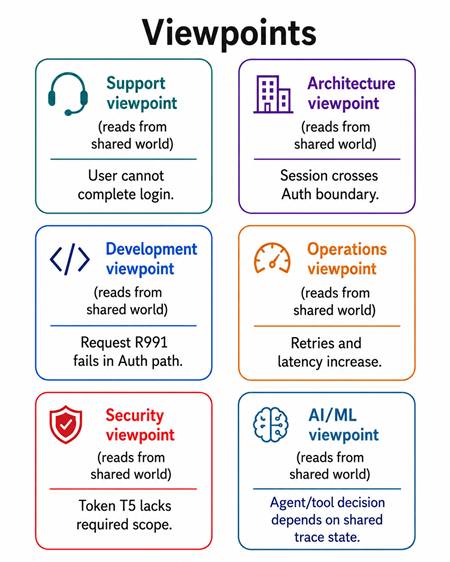
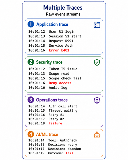
A single trace may reveal only a partial diagnostic world. An application trace may show requests and exceptions. A security trace may show tokens, scopes, and access decisions. An operations trace may show retries, timeouts, latency, and resource pressure. An AI/ML trace may show prompts, tool calls, agent decisions, model responses, and memory updates:

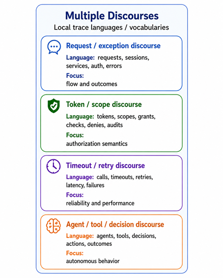
However, different traces are not only different in content. They may also belong to different Implementation Discourses. The earlier Implementation Discourse analysis pattern observes that non-trivial traces contain different discourses because components are written in different languages and follow different runtime environments, binary models, and interface frameworks. These implementation variations influence the structure, syntax, and semantics of trace messages; for example, .NET traces differ from file system driver traces or COM debugging messages:

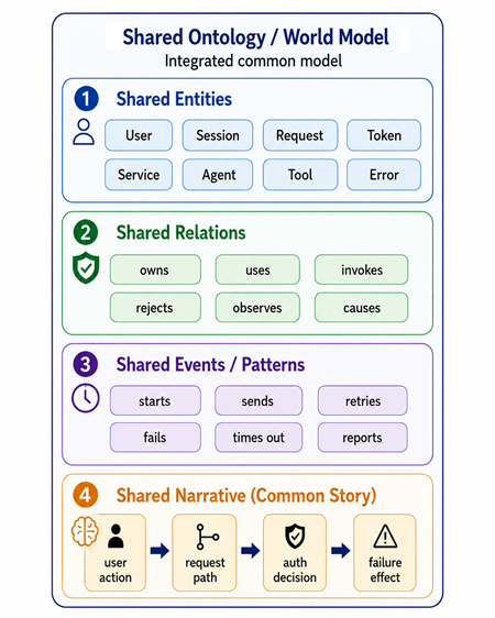
Trace World builds on this idea: it is a trace and log analysis pattern in which multiple traces, logs, telemetry streams, and diagnostic Trace Viewpoints contribute to a shared ontology of entities, relations, events, and narratives. The key idea is that multiple traces do not merely sit side by side. They share and enrich the same diagnostic ontology. As more traces are added, the Trace World becomes richer: new entities appear, existing entities are connected, relations become clearer, and the common narrative becomes more complete:

Therefore, Implementation Discourse is the local linguistic form of trace evidence, while Trace World is the shared world model that allows those local discourses to be translated, aligned, and used together. Implementation Discourse: How this component, runtime, framework, or language speaks in the trace. Trace World: How many such trace languages contribute to one shared diagnostic world. This also clarifies the relationship to Trace Ontology, which extracts entities, events, and relations from a trace, whereas Trace World allows multiple traces and multiple implementation discourses to share and enrich the same ontology.

Compared to Trace Viewpoints, which are different ways of reading the same trace world, and Implementation Discourses, which are different trace languages used to express evidence, Trace World is the common diagnostic world that persists when we move across both viewpoints and implementation discourses:

In agentic AI systems, this becomes especially important. Prompt traces, tool-call traces, memory traces, policy traces, model inference traces, application logs, and infrastructure telemetry may all speak different implementation discourses. Trace World provides the common diagnostic world where agents, tools, prompts, observations, memories, users, services, policies, and failures can be connected.

In summary, Trace World is the shared diagnostic world formed when multiple trace discourses enrich the same ontology, allowing analysts to move across viewpoints without losing entity identity, relations, or narrative continuity.

This analysis pattern is useful when:

• Several traces describe the same incident from different systems.
• Components use different trace languages, formats, and conventions.
• Different runtimes or frameworks produce structurally different messages, including Embedded Traces.
• The same entity appears under different names in different traces.
• A failure crosses application, infrastructure, security, data, or AI boundaries.
• A single trace discourse is insufficient to reconstruct the diagnostic story.

For constructing the Trace World, typical analysis steps may be these:

1. Identify the Implementation Discourse of each trace.
2. Extract Basic Facts from each discourse.
3. Identify local entities, events, and relations.
4. Map equivalent entities across discourses.
5. Merge them into a shared Trace World ontology.
6. Add relations that become visible only across traces.
7. Build a common narrative across implementation boundaries.
8. Use Trace Viewpoints to read the same world from different skill perspectives.

However, there might be some problems when using Trace World analysis pattern:

• Discourse isolation: each trace language remains separate.
• Translation gap: no mapping exists between local trace terms.
• Identity mismatch: the same entity has different names in different discourses.
• Semantic drift or incompatible Semantic Mappings: similar words mean different things in different traces.
• Partial or incompatible Trace Ontologies: one discourse lacks entities needed to explain another.
• Conflicting narrative: traces imply different causal stories.
• Unenriched world: traces are collected but not integrated.

- Dmitry Vostokov @ DumpAnalysis.org + TraceAnalysis.org -

In trace and log analysis, inductance and capacitance can serve as metaphors for two distinct forms of diagnostic behavior.

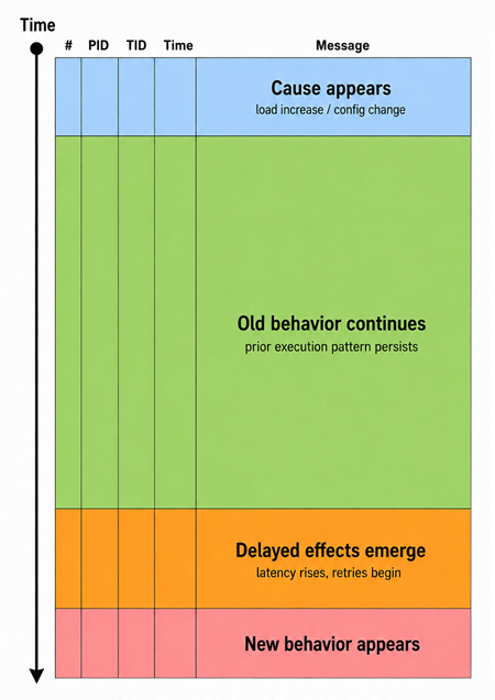
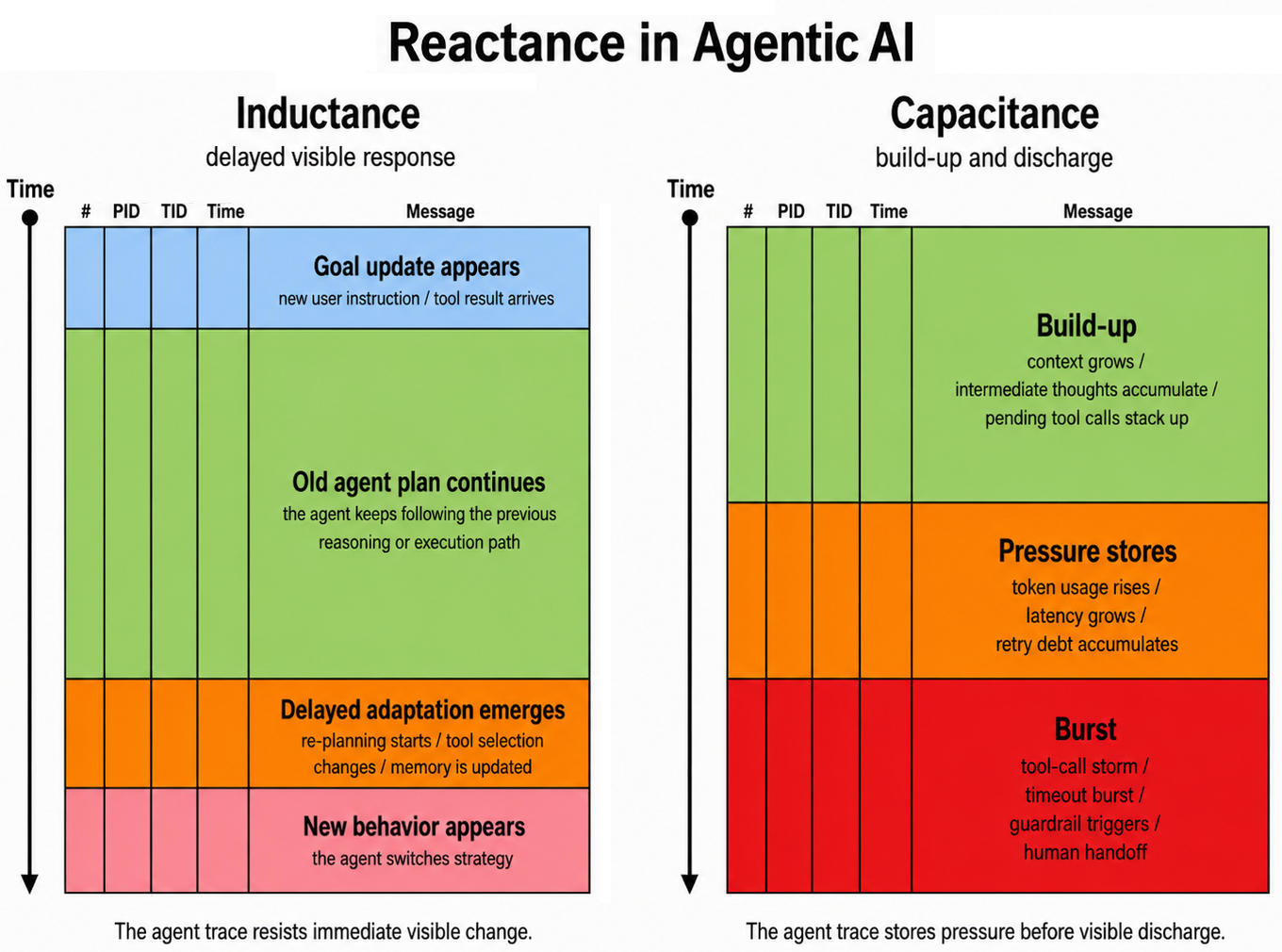
Trace Inductance is the tendency of a system to resist sudden changes in behavior. A new input, configuration change, request burst, or failure condition may not immediately appear in the trace as a new stable pattern. The existing execution flow has “momentum.” Threads, queues, retries, caches, locks, connection pools, batching, and background workers continue to reflect the previous state for some time:

Note that the cause may not be visible in the trace or log but may come from another trace and log, similar to Paratext in memory analysis.

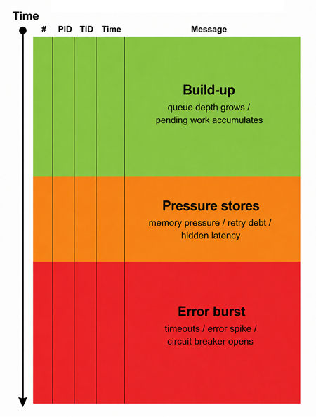
Trace Capacitance is the tendency of a system to accumulate diagnostic potential before a visible discharge occurs. The trace or log may look normal while internal state, queues, memory pressure, retry debt, latency, pending work, or error counters are accumulating. Then the system suddenly emits a burst of Error Messages, warnings, Timeouts, or Phase Transitions.

In summary, Trace Inductance explains delayed behavioral response, and Trace Capacitance explains delayed behavioral manifestation. The former asks: Why did the trace not change immediately after the cause? The latter asks: What was accumulating before the visible failure? Together they help avoid a common mistake: assuming that the first visible error is the real beginning of the problem. In many systems, the cause may appear before the symptom, because of inductance, and the symptom may appear suddenly because of capacitance.

We introduce Trace Reactance as a good umbrella analysis pattern name, with Trace Inductance and Trace Capacitance as two specializations of this pattern: Trace Reactance describes how diagnostic signals are delayed, smoothed, accumulated, or released by the system structure before becoming visible in traces and logs.

An agentic AI fits naturally here, too: agents accumulate context debt, token pressure, and retry state before a sudden degradation in output or a tool-call cascade both inductance and capacitance effects, for example (click on image to enlarge):

- Dmitry Vostokov @ DumpAnalysis.org + TraceAnalysis.org -

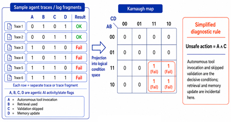
Large traces and logs often contain many combinations of conditions. The analyst sees many individual events but struggles to see which combinations are essential and which are redundant, equivalent, or adjacent manifestations of the same underlying behavior. The trace appears complex because the diagnostic space is fragmented into many small observations.

Karnaugh Map analysis pattern is useful when trace or log fragments can be classified by several binary or categorical dimensions, for example, distinctive features of Marked Messages. We project events into a structured logical space, similar to how a Karnaugh map projects Boolean combinations into an adjacency-preserving logical grid. Grouping cells in this grid simplifies the apparent complexity of many observed failure combinations into a minimal Boolean diagnostic condition, separating essential root cause dimensions from incidental ones that vary freely without affecting the outcome.

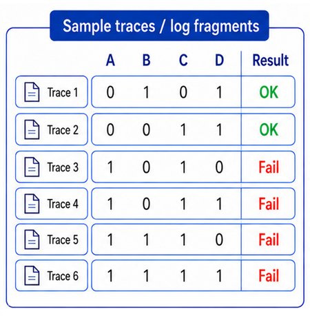
For example, suppose we analyze failures using four binary dimensions:

• A - Auth token expired
• B - Cache miss
• C - Backend timeout
• D - Retry attempt

We collected many traces for both working and non-working (failure) cases, and at first, it looks like there are four different failure cases:

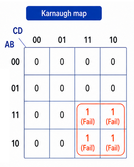
But in Karnaugh-map form, these four cases form one group. The varying dimensions are B and D, while A and C remain constant:

So the simplified diagnostic condition is: failure occurs when the auth token expires and the backend times out, regardless of cache state or retry state. Or, in Boolean-like form: Failure = A ∧ C. This means cache misses and retries are not root discriminators here. They are incidental dimensions.

Here is a similar example for agentic AI:

- Dmitry Vostokov @ DumpAnalysis.org + TraceAnalysis.org -

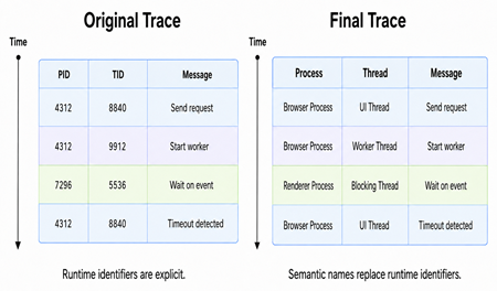
Semantic Mapping is the trace and log analysis pattern where opaque runtime identifiers such as PIDs, TIDs, request IDs, handles, or session IDs are renamed or mapped to semantically meaningful diagnostic entities such as UI Thread, Worker Thread, Client Process, Blocking Thread, or Failed Request:

Additionally, in Semantic Mapping, we cannot only rename identifier values but also rename the Trace Schema itself, for example, changing column headers such as PID to Process and TID to Thread.

This analysis pattern differs from Trace Field, which is a mapping/function from trace messages to some other domain. It does not necessarily rewrite the trace presentation itself, but it may add additional ATID c to the Trace Schema. It is also different from Semantic Field, which is a semantic category/codomain/class into which trace messages are grouped, which is more about the meaningful domain of classification, not about rewriting trace labels. On the contrary, Semantic Mapping is a representation transformation that rewrites the trace into a more meaningful diagnostic form. It operates at two levels: instance level, renaming actual values, and schema level, renaming the fields/headers themselves.

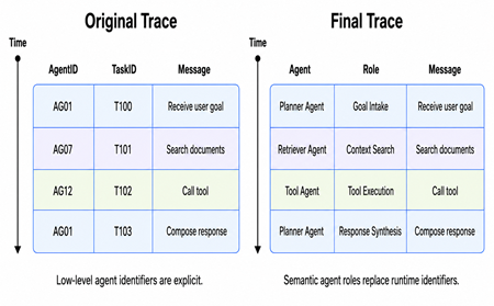
Here is another example adapted to agentic AI:

Using mathematical analogies, Semantic Mapping is essentially a readability-preserving isomorphism: the structural information is unchanged, but a human (or AI analyst) now works in a named, meaningful coordinate system rather than an anonymous numeric one.

- Dmitry Vostokov @ DumpAnalysis.org + TraceAnalysis.org -