Software Diagnostics Library

The Trace Multiphysics analysis pattern applies several Trace Fields to the same sequence of trace messages and studies both their individual strengths and their interactions. A Trace Field associates every message in a trace domain M with a value in some analytical range T. Although the field is defined over M, its values need not be extracted solely from that trace. A value may be derived from the message itself, inferred from its surrounding context, or assigned using correlated evidence from other traces, logs, metrics, memory dumps, snapshots, models, or external knowledge sources. The value does not need to be numerical, although numerical or ordered values are useful when field strength must be visualized. For example, one field may represent execution significance, another resource pressure, and a third semantic or user-visible importance:

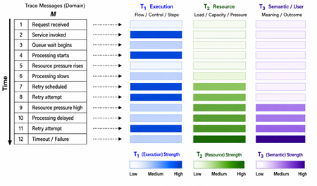
However, Trace Multiphysics is not merely the display of several independent Trace Fields: its essential feature is their coupling. A change in one field may affect another field. For example, increased resource pressure may slow execution. Slower execution may trigger retries. Repeated retries may further increase resource pressure. Eventually, the combined effect may change the semantic or user-visible outcome. The coupling diagram represents these relationships, and arrow thickness indicates coupling strength:

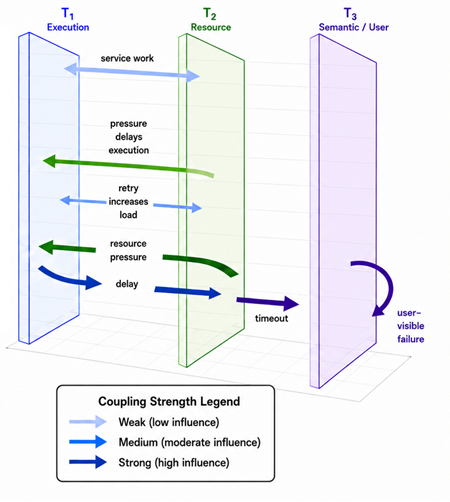
A simple conceptual form is: C_ij​(m)=g(f_i​(m), f_j​(m), R_ij​(m)), where f_i​: M → T_i and f_j​: M → T_j, f_i(m) and f_j(m) are the strengths or values of fields i and j at message m, C_ij(m) is the coupling between fields i and j at message m, and R_ij(m) represents evidence of an interaction between the two fields, obtained from the trace itself or from correlated diagnostic sources. This formula defines coupling at message m. More generally, a coupling may relate field values at different messages when the influence is delayed or propagated through the trace: C_ij​(m_a, m_b)=g(f_i​(m_a), f_j​(m_b), R_ij​(m_a, m_b)), where m_a ⪯ m_b. Here, R_ij​(m_a, m_b) represents evidence relating the value f_i(m_a) of field i to the value f_j(m_b) of field j, whether that evidence is contained in the primary trace or supplied through correlated artifacts. High values in two fields do not automatically establish strong coupling. The available diagnostic evidence must also support the conclusion that one field influences, constrains, amplifies, transforms, or explains the other. Such evidence may occur in the primary trace or in correlated traces, logs, metrics, snapshots, models, or other diagnostic artifacts:

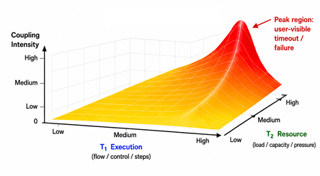
The mapping f_i is defined over the trace domain M, but its construction may depend on evidence outside M. A more explicit form is: f_i(m) = h_i(m, E_i(m)), where E_i(m) is the evidence associated with message m. This evidence may come from the message itself, nearby messages, other traces or logs, metrics, snapshots, memory dumps, learned models, or other correlated diagnostic sources. Correlation may be established through timestamps, identifiers, causal links, shared entities, execution context, or other relations.

When no ordinary field value can be assigned, T_i may include special values representing unknown, unavailable, or not applicable, preserving the definition of the field over the complete trace domain.

In computational modeling, multiphysics simulation studies several aspects of a physical system and their interactions simultaneously. A model may combine thermal, structural, fluid, electromagnetic, or other processes, together with the coupling and boundary conditions between them. Trace Multiphysics transfers this structural principle to software diagnostics. The analogy does not imply that all software behavior should be described by physical equations. Instead, it provides a disciplined way to analyze several interacting dimensions without reducing the incident to one isolated perspective.

The connection is especially appropriate in software diagnostics because software can be its own model. Software execution states and execution artifacts can be copied, preserved, replayed, or analyzed independently. Traces, logs, metrics, memory dumps, and snapshots are symbolic and digital artifacts produced by the software system itself. In this diagnostic sense, software performs a form of self-simulation: its execution generates artifacts that model selected aspects of its own structure and behavior. A trace is not a complete reproduction of the running system. It is a selective, instrumented self-model. Different Trace Fields map messages in that self-model to values in different analytical ranges, each representing a distinct analytical dimension. Some values may be extracted directly from the trace, while others may be inferred, enriched, or projected from correlated traces, logs, metrics, memory dumps, snapshots, models, or external knowledge. Trace Multiphysics studies those fields together and examines how they interact. Thus, multiphysics simulation models several interacting physical processes, whereas Trace Multiphysics analyzes several interacting fields defined over a software-generated model of software behavior and potentially enriched from other diagnostic sources.

Trace Field provides the foundational assignment or mapping from trace messages to values in one analytical range. The field is defined over a selected trace domain, but the evidence used to assign its values may originate inside or outside that domain. Trace Multiphysics extends this principle by applying several Trace Fields to the same trace domain and analyzing their simultaneous values, changing strengths, overlap at individual messages, dependencies, feedback loops, coupling strengths, and combined explanatory effects. The relationship can be summarized as follows: Trace Field maps trace messages to values in one analytical range, while Trace Multiphysics studies several coupled Trace Fields defined over the same trace domain, with their values potentially derived from or enriched by evidence from multiple diagnostic sources.

Trace Multiphysics also connects to several recent analysis patterns. In Trace Reactance, inductive and capacitive effects can be understood as specific forms of inter-field coupling and temporal distortion produced by interacting state fields. Karnaugh Map is also multidimensional but primarily Boolean and combinatorial, whereas Trace Multiphysics accommodates continuous or graded fields, propagation, and feedback loops. Trace World may provide a broader shared diagnostic context in which coupled Trace Fields are interpreted. Bethe Ansatz is a constrained form of Trace Multiphysics in which global behavior is reconstructed from composable pairwise interaction motives.

The pattern is particularly relevant to AI/ML and agentic AI systems. Multiphysics approaches in machine learning usually apply ML to coupled physical processes or incorporate multiple physical priors into learning. Multiphysics-Inspired AI/ML Observability and Diagnostics, by contrast, treats the AI/ML system itself as a collection of interacting analytical fields, including data, optimization, information, computation, uncertainty, control, and semantic outcome fields, defined over a common trace domain constructed from correlated training, inference, and operational events. Its observability aspect concerns the instrumentation, correlation, and enrichment required to construct these fields from training logs, model evaluations, infrastructure metrics, distributed traces, tool-call records, user interactions, safety assessments, and other evidence sources. Its diagnostic aspect concerns how fields interact through their values and couplings, how disturbances propagate across fields, how feedback loops emerge among them, and how their combined effects produce system-level behavior.

In an agentic AI system, for example, increased tool latency may cause retries. Retries may enlarge the accumulated context and increase computational pressure. Context growth may change the relative prominence of relevant information and increase uncertainty, affecting planning, tool selection, and the final semantic outcome. A degraded outcome may provoke further retries, creating a reinforcing feedback loop. Observability provides the correlated evidence needed to construct, expose, and track these fields, while diagnostics analyzes their values and couplings to explain the resulting agent behavior. The behavior cannot be explained adequately by any one field in isolation.

In summary, Trace Multiphysics is a trace and log analysis pattern that examines several Trace Fields defined over the same trace domain, whether their values are derived from that trace alone or assigned using correlated evidence from other diagnostic sources. It studies the immediate, delayed, reinforcing, constraining, transforming, and explanatory couplings through which their combined behavior emerges. Multiphysics-Inspired AI/ML Observability and Diagnostics extends this principle to AI/ML and agentic systems: observability constructs and exposes the relevant fields from distributed evidence, while diagnostics analyzes their interactions and explains the emergent system behavior.

- Dmitry Vostokov @ DumpAnalysis.org + TraceAnalysis.org -

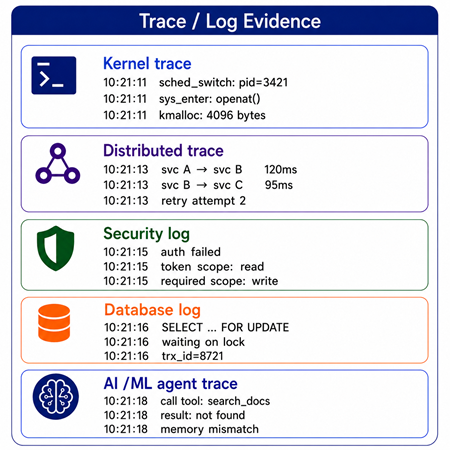
Even when all relevant events are present in traces and logs, they may still remain opaque because the analyst lacks the specialized skill needed to interpret their messages, abstractions, timing, domain vocabulary, failure semantics, or their role in the broader Trace World:

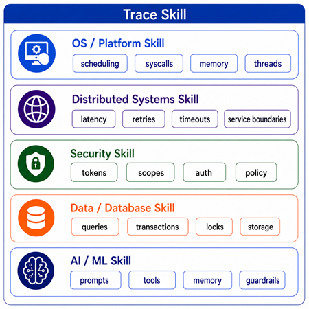
Trace Skill is a trace and log analysis pattern in which successful interpretation depends on a specific skill set required by the trace domain or Trace Ontology:

Some traces can be read with general diagnostic experience, especially if domain-independent analysis patterns are used. Others require specialist knowledge:

• Kernel tracing requires OS internals skill.
• Distributed traces require distributed systems skill.
• Database logs require query, transaction, and storage skill.
• Security logs require identity, policy, token, and threat-modeling skill.
• ML/AI traces require model, prompt, embedding, evaluation, and agentic workflow skill.
• Performance traces require latency, contention, scheduling, and resource-analysis skill.
• Business-process traces require domain workflow knowledge.

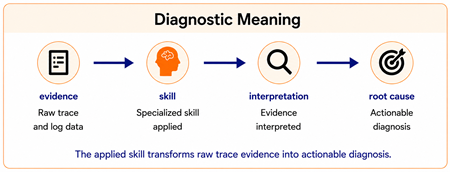
The same trace may therefore be simple for one analyst and almost invisible for another. Even the same analysis pattern may be applied differently. The problem is not the absence of data but the absence of the interpretive skill needed to turn trace data into diagnostic meaning:

Trace Skill analysis pattern may be useful in the following situations:

• The trace contains relevant evidence, but the analyst does not recognize it.
• Messages are dismissed as noise because their domain meaning is unknown.
• A team reads only the parts of the trace matching its own expertise.
• Different specialists disagree because each understands only one layer.
• The trace crosses technical boundaries: application, infrastructure, security, data, ML, business logic.
• The incident is repeatedly escalated because no one possesses the required combination of skills.

Compared to other analysis patterns, Trace Viewpoints are perspectives from which the trace is read. Trace Skill is the competence needed to read from a viewpoint correctly. So a viewpoint can be chosen quickly, but a skill has to be possessed, acquired, or borrowed from someone else. Trace World allows movement across skill sets by creating a common diagnostic language, but Trace Skill explains why this is necessary: traces are often multi-skill artifacts. No single narrow skill may be enough. The analyst either needs multiple skills or needs to collaborate across skill boundaries using a shared Trace World.

We can also say that Trace Skill is needed to navigate traces and logs and their Trace World. Trace World provides the shared diagnostic terrain constructed from trace and log evidence, entities, relations, events, timelines, and viewpoints. Trace Skill is the specialized competence required to navigate both the raw evidence and the reconstructed world accurately, recognize relevant signals, switch between viewpoints, and avoid misinterpretation.

In summary, Trace Skill is a trace and log analysis pattern in which decisive diagnostic evidence can only be recognized by the appropriate specialist skill set.

- Dmitry Vostokov @ DumpAnalysis.org + TraceAnalysis.org -

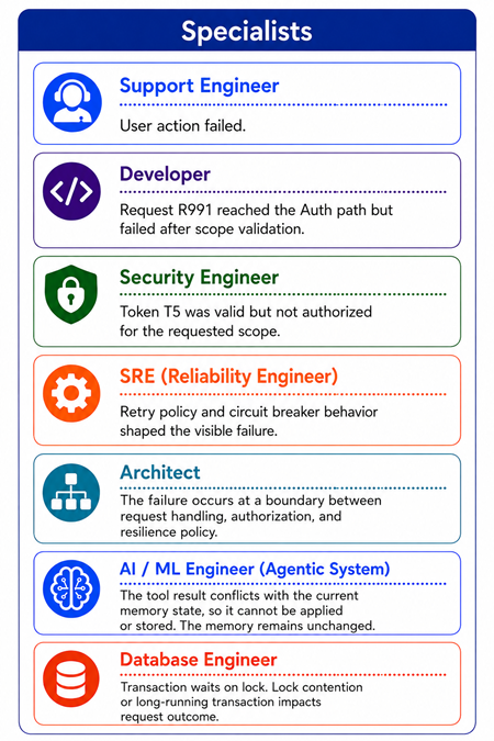
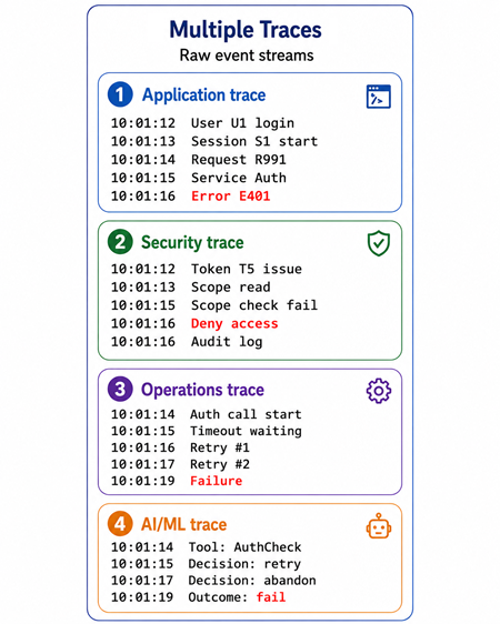
A single trace may reveal only a partial diagnostic world. An application trace may show requests and exceptions. A security trace may show tokens, scopes, and access decisions. An operations trace may show retries, timeouts, latency, and resource pressure. An AI/ML trace may show prompts, tool calls, agent decisions, model responses, and memory updates:

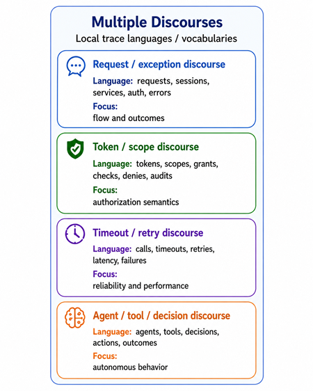
However, different traces are not only different in content. They may also belong to different Implementation Discourses. The earlier Implementation Discourse analysis pattern observes that non-trivial traces contain different discourses because components are written in different languages and follow different runtime environments, binary models, and interface frameworks. These implementation variations influence the structure, syntax, and semantics of trace messages; for example, .NET traces differ from file system driver traces or COM debugging messages:

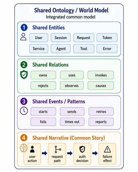
Trace World builds on this idea: it is a trace and log analysis pattern in which multiple traces, logs, telemetry streams, and diagnostic Trace Viewpoints contribute to a shared ontology of entities, relations, events, and narratives. The key idea is that multiple traces do not merely sit side by side. They share and enrich the same diagnostic ontology. As more traces are added, the Trace World becomes richer: new entities appear, existing entities are connected, relations become clearer, and the common narrative becomes more complete:

Therefore, Implementation Discourse is the local linguistic form of trace evidence, while Trace World is the shared world model that allows those local discourses to be translated, aligned, and used together. Implementation Discourse: How this component, runtime, framework, or language speaks in the trace. Trace World: How many such trace languages contribute to one shared diagnostic world. This also clarifies the relationship to Trace Ontology, which extracts entities, events, and relations from a trace, whereas Trace World allows multiple traces and multiple implementation discourses to share and enrich the same ontology.

Compared to Trace Viewpoints, which are different ways of reading the same trace world, and Implementation Discourses, which are different trace languages used to express evidence, Trace World is the common diagnostic world that persists when we move across both viewpoints and implementation discourses:

In agentic AI systems, this becomes especially important. Prompt traces, tool-call traces, memory traces, policy traces, model inference traces, application logs, and infrastructure telemetry may all speak different implementation discourses. Trace World provides the common diagnostic world where agents, tools, prompts, observations, memories, users, services, policies, and failures can be connected.

In summary, Trace World is the shared diagnostic world formed when multiple trace discourses enrich the same ontology, allowing analysts to move across viewpoints without losing entity identity, relations, or narrative continuity.

This analysis pattern is useful when:

• Several traces describe the same incident from different systems.
• Components use different trace languages, formats, and conventions.
• Different runtimes or frameworks produce structurally different messages, including Embedded Traces.
• The same entity appears under different names in different traces.
• A failure crosses application, infrastructure, security, data, or AI boundaries.
• A single trace discourse is insufficient to reconstruct the diagnostic story.

For constructing the Trace World, typical analysis steps may be these:

1. Identify the Implementation Discourse of each trace.
2. Extract Basic Facts from each discourse.
3. Identify local entities, events, and relations.
4. Map equivalent entities across discourses.
5. Merge them into a shared Trace World ontology.
6. Add relations that become visible only across traces.
7. Build a common narrative across implementation boundaries.
8. Use Trace Viewpoints to read the same world from different skill perspectives.

However, there might be some problems when using Trace World analysis pattern:

• Discourse isolation: each trace language remains separate.
• Translation gap: no mapping exists between local trace terms.
• Identity mismatch: the same entity has different names in different discourses.
• Semantic drift or incompatible Semantic Mappings: similar words mean different things in different traces.
• Partial or incompatible Trace Ontologies: one discourse lacks entities needed to explain another.
• Conflicting narrative: traces imply different causal stories.
• Unenriched world: traces are collected but not integrated.

- Dmitry Vostokov @ DumpAnalysis.org + TraceAnalysis.org -

A typical trace or log is a detailed narrative, and one of the first analysis tasks is to check whether the expected Basic Facts are present: user name, machine name, process, component, time, operation, resource, or other problem-description facts. If those facts are absent or inconsistent, the trace may have been collected at the wrong time, on the wrong system, or under different conditions:

However, vocabulary alone is not enough. A trace may contain all expected words and identifiers, yet the analyst (human or AI) may still not understand what kind of things they are, how they relate, and what diagnostic roles they play. Usernames, process IDs, request IDs, sessions, endpoints, file names, transactions, queues, locks, models, agents, function and tool calls, or error messages are trace entities with roles and relationships. Trace Ontology is a trace and log analysis pattern that identifies the domain entities, classes, relations, and constraints, both explicit and implicit, in trace messages. It turns raw trace vocabulary into a practical structured diagnostic model:

Therefore, Trace Ontology extends Basic Facts from vocabulary recognition to structured diagnostic representation. In summary, Basic Facts answer the following question: What vocabulary from the problem description is visible in the trace or log? Trace Ontology answers: What kinds of things exist in this trace, how are they related, and what can be inferred from those relations?

Also, Trace Ontology, as a representational model, can be coupled with Semantic Mapping, a presentation transformation that relabels opaque identifiers with meaningful names. Note that trace ontologies may exist before traces are collected. In such a case, they simplify the analysis.

- Dmitry Vostokov @ DumpAnalysis.org + TraceAnalysis.org -

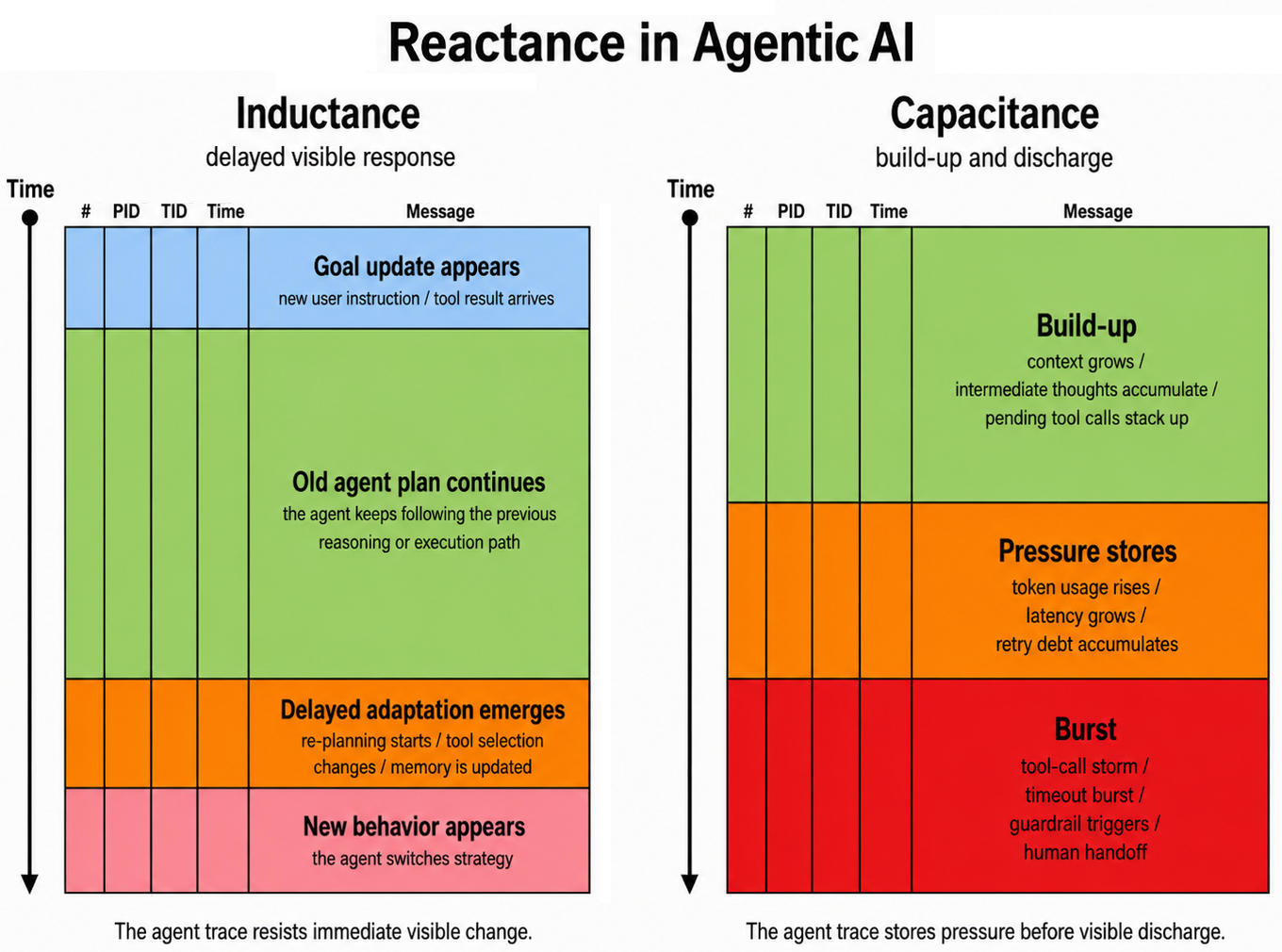
In trace and log analysis, inductance and capacitance can serve as metaphors for two distinct forms of diagnostic behavior.

Trace Inductance is the tendency of a system to resist sudden changes in behavior. A new input, configuration change, request burst, or failure condition may not immediately appear in the trace as a new stable pattern. The existing execution flow has “momentum.” Threads, queues, retries, caches, locks, connection pools, batching, and background workers continue to reflect the previous state for some time:

Note that the cause may not be visible in the trace or log but may come from another trace and log, similar to Paratext in memory analysis.

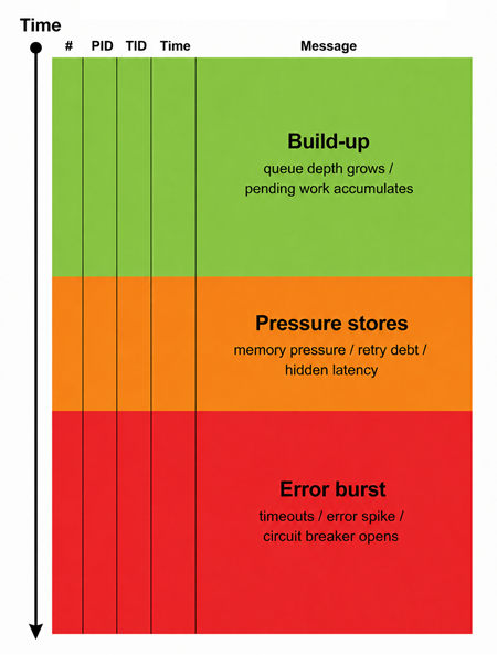
Trace Capacitance is the tendency of a system to accumulate diagnostic potential before a visible discharge occurs. The trace or log may look normal while internal state, queues, memory pressure, retry debt, latency, pending work, or error counters are accumulating. Then the system suddenly emits a burst of Error Messages, warnings, Timeouts, or Phase Transitions.

In summary, Trace Inductance explains delayed behavioral response, and Trace Capacitance explains delayed behavioral manifestation. The former asks: Why did the trace not change immediately after the cause? The latter asks: What was accumulating before the visible failure? Together they help avoid a common mistake: assuming that the first visible error is the real beginning of the problem. In many systems, the cause may appear before the symptom, because of inductance, and the symptom may appear suddenly because of capacitance.

We introduce Trace Reactance as a good umbrella analysis pattern name, with Trace Inductance and Trace Capacitance as two specializations of this pattern: Trace Reactance describes how diagnostic signals are delayed, smoothed, accumulated, or released by the system structure before becoming visible in traces and logs.

An agentic AI fits naturally here, too: agents accumulate context debt, token pressure, and retry state before a sudden degradation in output or a tool-call cascade both inductance and capacitance effects, for example (click on image to enlarge):

- Dmitry Vostokov @ DumpAnalysis.org + TraceAnalysis.org -

Large traces and logs often contain many combinations of conditions. The analyst sees many individual events but struggles to see which combinations are essential and which are redundant, equivalent, or adjacent manifestations of the same underlying behavior. The trace appears complex because the diagnostic space is fragmented into many small observations.

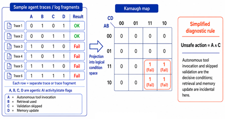
Karnaugh Map analysis pattern is useful when trace or log fragments can be classified by several binary or categorical dimensions, for example, distinctive features of Marked Messages. We project events into a structured logical space, similar to how a Karnaugh map projects Boolean combinations into an adjacency-preserving logical grid. Grouping cells in this grid simplifies the apparent complexity of many observed failure combinations into a minimal Boolean diagnostic condition, separating essential root cause dimensions from incidental ones that vary freely without affecting the outcome.

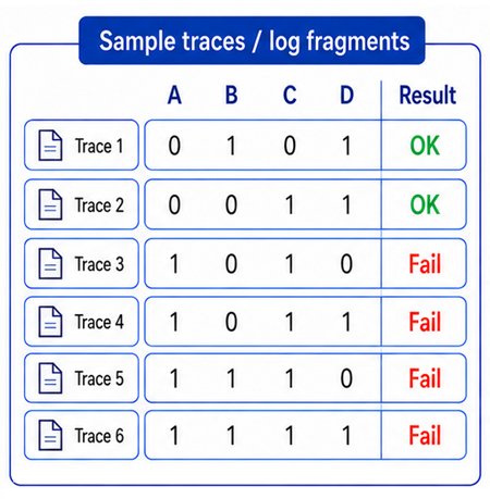
For example, suppose we analyze failures using four binary dimensions:

• A - Auth token expired
• B - Cache miss
• C - Backend timeout
• D - Retry attempt

We collected many traces for both working and non-working (failure) cases, and at first, it looks like there are four different failure cases:

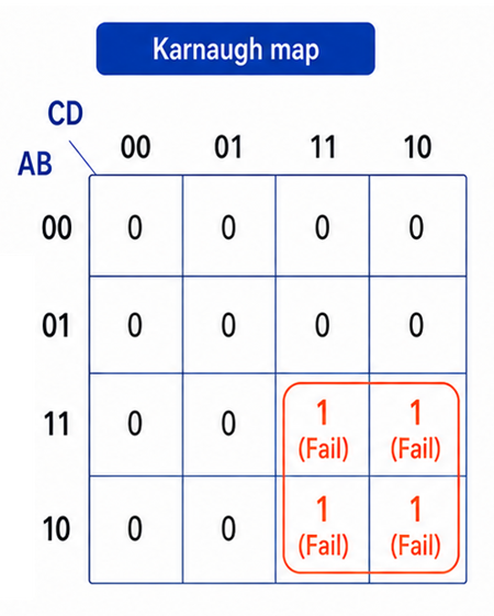
But in Karnaugh-map form, these four cases form one group. The varying dimensions are B and D, while A and C remain constant:

So the simplified diagnostic condition is: failure occurs when the auth token expires and the backend times out, regardless of cache state or retry state. Or, in Boolean-like form: Failure = A ∧ C. This means cache misses and retries are not root discriminators here. They are incidental dimensions.

Here is a similar example for agentic AI:

- Dmitry Vostokov @ DumpAnalysis.org + TraceAnalysis.org -

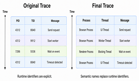
Semantic Mapping is the trace and log analysis pattern where opaque runtime identifiers such as PIDs, TIDs, request IDs, handles, or session IDs are renamed or mapped to semantically meaningful diagnostic entities such as UI Thread, Worker Thread, Client Process, Blocking Thread, or Failed Request:

Additionally, in Semantic Mapping, we cannot only rename identifier values but also rename the Trace Schema itself, for example, changing column headers such as PID to Process and TID to Thread.

This analysis pattern differs from Trace Field, which is a mapping/function from trace messages to some other domain. It does not necessarily rewrite the trace presentation itself, but it may add additional ATID c to the Trace Schema. It is also different from Semantic Field, which is a semantic category/codomain/class into which trace messages are grouped, which is more about the meaningful domain of classification, not about rewriting trace labels. On the contrary, Semantic Mapping is a representation transformation that rewrites the trace into a more meaningful diagnostic form. It operates at two levels: instance level, renaming actual values, and schema level, renaming the fields/headers themselves.

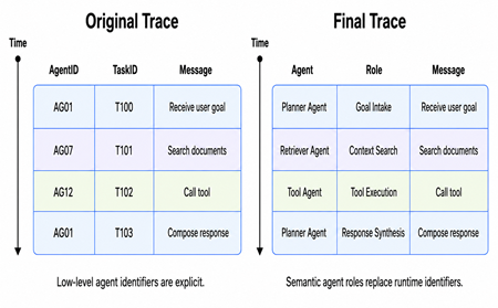
Here is another example adapted to agentic AI:

Using mathematical analogies, Semantic Mapping is essentially a readability-preserving isomorphism: the structural information is unchanged, but a human (or AI analyst) now works in a named, meaningful coordinate system rather than an anonymous numeric one.

- Dmitry Vostokov @ DumpAnalysis.org + TraceAnalysis.org -

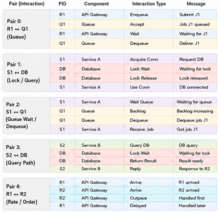
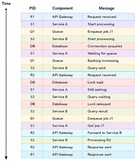
Usually, in traces and logs, messages from different components are highly interleaved. Direct chronological reading may cause confusion because every component’s Adjoint Thread of Activity appears entangled with every other one:

Bethe Ansatz analyzes such a trace by treating requests, threads, agents, transactions, or log-producing entities as “quasi-particles” whose global behavior can be reconstructed from many local pairwise interactions. The inspiration for the pattern name comes from Bethe ansatz, introduced by Hans Bethe in 1931. In physics, it is a method for constructing exact solutions of certain many-body systems: in integrable systems, complex many-body scattering can be represented through factorized two-body scattering processes. In trace analysis, we often face a “many-body” problem: many requests, threads, services, queues, locks, agents, retries, callbacks, and timeouts interact within a single shared diagnostic space. Instead of trying to understand the whole trace as one monolithic event cloud, we decompose it into stable activity lines and pairwise encounters that may explain the global behavior:

The Bethe ansatz has many forms, including coordinate, algebraic, analytic, functional, nested, and thermodynamic variants. For this pattern, the most useful metaphor is the coordinate Bethe ansatz: represent the global state by positions of entities and interaction effects between them. We have the following analogies:

• Particle/excitation: request, thread, transaction, agent, session, workflow
• Coordinate: timestamp, component, hop number, queue position, memory address, trace span
• Momentum/rapidity: (activity) rate, latency class, retry rhythm, priority, causal direction
• Two-body scattering: (pairwise interaction) lock contention, queue wait, API call, resource conflict
• Scattering phase shift: delay, reordered event, changed state, timeout extension, retry offset
• Factorized many-body scattering: whole trace explained as composition of pairwise effects
• Bethe equations: consistency constraints imposed by loops, boundaries, cycles, repeated paths
• Non-integrability: residual behavior not explainable by pairwise interactions

Interactions can be found among Motifs, Macrofunctions, and actors of Activity Theatre.

We suggest the following diagnostic analysis procedure:

1. Identify trace quasi-particles that preserve identity across the trace.
2. Choose a coordinate system: the trace can be read through coordinates other than time.
3. Detect pairwise encounters: look for places where two entities interact; these are diagnostic “scattering” events.
4. Estimate phase shifts where a pairwise encounter often changes the apparent trajectory of an activity. The phase shift is the observable deformation caused by interaction.
5. Test factorization by asking the question: Can the global anomaly be explained as a product of pairwise interactions?

If the answer to the last question is yes, then the system is “Bethe-like”: complex but decomposable. If the answer is no, there may be a true many-body effect, such as shared cache collapse, global scheduler starvation, cascading timeout storm, distributed deadlock, correlated retry amplification, emergent agentic loop, or resource exhaustion caused by collective behavior.

Additionally, we can form a Motivic Trace from the resulting pairwise interaction layers. Motivic Trace compresses a trace into explanatory motives. Bethe Ansatz compresses a trace into pairwise interaction motives whose composition reconstructs the observed global behavior. In this sense, Bethe Ansatz can be viewed as a structured route to Motivic Trace: first decompose the tangled chronological trace into stable activity lines and pairwise encounters; then integrate those encounters into higher-level explanatory motives such as queue delay, database lock wait, retry ordering, and response ordering. In summary: Motivic Trace is the broader compression pattern; Bethe Ansatz is a pairwise-factorized way to build it.

A historical note: this analysis pattern also extends physical analogies of debugging.

- Dmitry Vostokov @ DumpAnalysis.org + TraceAnalysis.org -

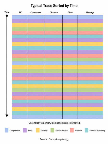
Usually, software traces and logs are sorted by time.

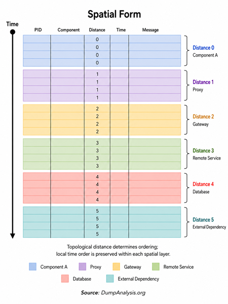
Spatial Form is a specialized Sorted Trace in which trace or log messages are sorted by spatial, topological, or diagnostic proximity to a chosen origin component, device, process, service, or subsystem. Instead of reading the trace solely as a chronological sequence, we choose a diagnostic origin and arrange messages by their distance from that origin. Within each distance layer, the original local time order may still be preserved.

The pattern name comes from Joseph Frank’s The Idea of Spatial Form that is associated with reading narrative structure through juxtaposition and relational arrangement rather than only through linear chronological progression; the concept was introduced into literary discussion through his 1945 essay and later collected with reconsiderations in his book.

Sorted Trace is the more general pattern: messages are sorted according to some attribute value, for example, by TID, ATID, message type, message invariants, or message data.

For Spatial Trace, the distance may come from network topology, service dependency graph, component containment, process/thread ownership, device hierarchy, pipeline stage distance, proxy/gateway chain, address-space relation, storage or shard topology, causal adjacency, and many others. The resulting trace is not anti-temporal. It is spatially primary and temporally secondary.

Spatial Trace analysis pattern may help answer these questions: What happened around this proxy? Which nearby component first showed abnormal behavior? How did the request propagate outward? Was the fault local, adjacent, or remote? It may help distinguish local symptoms, adjacent symptoms, downstream effects, remote dependencies, and external causes. It gives the trace a layered diagnostic structure and spatial Layered Periodization. The pattern is therefore both a sorting technique and a reading strategy.

This pattern is especially useful for distributed systems, microservices, network devices, storage stacks, cloud control planes, request pipelines, proxies, gateways, and agentic AI workflows where activity is spread across many components.

- Dmitry Vostokov @ DumpAnalysis.org + TraceAnalysis.org -

This is a Linux pattern variant of the Windows Spiking Interrupts memory analysis pattern. The Windows pattern describes high interrupt and DPC activity that causes perceived freezes, response lag, or high kernel CPU time; the original pattern uses per-processor interrupt counts, DPC/interrupt time, and DPC queue data, and stresses comparisons with a normal system because raw counters depend on uptime.

On Linux, the closest mapping is (including associated Paratext):

Hardware interrupts - hard IRQs, vectors, MSI/MSI-X, per-device IRQ lines

DPC - softirq, tasklet, NAPI poll, threaded IRQ, sometimes workqueue

DPC delegate thread / idle-context DPC execution - ksoftirqd/N, irq/<irq>-<name>, kworker/*

!prcb, DPC counts, interrupt time - /proc/interrupts, /proc/softirqs, /proc/stat, crash> irq -s, stacks, logs

Note: The mapping of DPC delegate thread / idle-context DPC execution to kworker/* is an approximation. Workqueues run in kernel thread context and can execute deferred work similarly to how idle-context DPCs offload work from the interrupt path, but workqueues are a general-purpose deferral mechanism, not specifically an interrupt bottom-half mechanism. Unlike softirqs and tasklets, which exist primarily to defer interrupt handler work, a kworker stall may have nothing to do with interrupt pressure. When investigating spiking interrupt symptoms, kworker threads appearing in stacks should be treated as a secondary signal only, and their work items examined individually (via crash> bt on the kworker thread) to determine whether they originate from IRQ or softirq context before drawing conclusions about interrupt-driven CPU saturation.

As we see, Linux has no exact DPC object model. The strongest Linux analogy is when a CPU is consumed by hard IRQs and/or interrupt-related bottom-half work, such as softirqs, tasklets, NAPI polling, threaded IRQs, or interrupt-originated workqueue processing.

The crash tool irq command and its various options may show when a single CPU is absorbing a device interrupt stream:

crash> irq -s
           CPU0       CPU1
[...]
 77:     513461          0  MSI io-request
[...]

Then we check whether that CPU was also the crash CPU, a soft-lockup CPU, an RCU-stall CPU, or the CPU running ksoftirqd/N using the follow-up commands such as:

crash> ps | grep -E "ksoftirqd|irq/|kworker|rcu"

crash> runq

crash> bt -a

crash> bt -E

The last command searches IRQ stacks, and on x64 also exception stacks, for possible exception frames on supported architectures

If ksoftirqd/* is running or runnable and CPU* also has rapidly accumulated NET_RX, NET_TX, BLOCK, TIMER, or RCU softirq work, that is the Linux equivalent of DPC pressure. softirqs are deferred interrupt work that can run after an interrupt handler or from ksoftirqd; when limits are reached, pending softirqs are run from ksoftirqd. Also, ksoftirqd/* executes softirq handlers when threaded or under heavy load, and irq/<irq>-<name> handles threaded interrupts. See: https://docs.kernel.org/admin-guide/kernel-per-CPU-kthreads.html

You can also see interrupt-pressure symptoms in the kernel log:

crash> log

Typical diagnostic messages include these fragments:

watchdog: BUG: soft lockup - CPU#N stuck
NMI watchdog: Watchdog detected hard LOCKUP on cpu N
rcu: INFO: rcu_sched detected stalls on CPUs/tasks
irq XX: nobody cared
Disabling IRQ #XX
NETDEV WATCHDOG: ... transmit queue timed out

RCU stall logs are particularly useful because the kernel documentation explicitly lists CPUs looping with interrupts disabled, preemption disabled, bottom halves disabled, or periodic interrupt handlers taking too long as possible causes. It also says reproducible massive hard/soft interrupt cases can be narrowed using /proc/interrupts. See: https://docs.kernel.org/RCU/stallwarn.html

For RCU definition, see https://en.wikipedia.org/wiki/Read-copy-update

Below is the guide for collecting supplemental paratext information from the live system:

// Hard IRQ distribution

cat /proc/interrupts
watch -n 1 cat /proc/interrupts

/proc/interrupts records the number of interrupts per CPU per I/O device and, on x64, also includes internal interrupts such as NMI, LOC, TLB, RES, and CAL. See: https://man7.org/linux/man-pages/man5/proc_interrupts.5.html

// SoftIRQ distribution

cat /proc/softirqs
watch -n 1 cat /proc/softirqs

Common rows include:

NET_RX      receive-side network pressure
NET_TX      transmit-side network pressure
BLOCK       block I/O completion pressure
IRQ_POLL    block polling pressure
TIMER       timer callback pressure
HRTIMER     high-resolution timer pressure
SCHED       scheduler/IPI/load-balancing pressure
RCU         RCU callback pressure
TASKLET     legacy driver deferred work

The /proc/stat softirq line reports the count of softirqs serviced since boot, and /proc/stat also reports CPU time spent servicing irqs and softirqs. See: https://www.kernel.org/doc/html/v6.9/filesystems/proc.html

// IRQ and softirq CPU time

awk '
/^cpu[0-9]/ {
printf "%s irq_jiffies=%s softirq_jiffies=%s\n", $1, $7, $8
}' /proc/stat

while true; do
date
awk '/^cpu[0-9]/ {printf "%s irq=%s softirq=%s\n",$1,$7,$8}' /proc/stat
sleep 1
done

High irq time points more toward hard interrupt handling. High softirq time points more toward deferred interrupt work such as NAPI, timers, block completions, scheduler softirqs, or RCU.

// IRQ affinity

Summary:

Spiking Interrupt activity is suspected when response latency or apparent freezes coincide with disproportionate hard IRQ or softirq activity on one or more CPUs. In a core dump, the pattern appears as high per-CPU IRQ counters, IRQ-affinity skew, active IRQ/softirq/ksoftirqd/threaded-IRQ stacks, and possible watchdog or RCU-stall messages. In live /proc, the pattern appears as rapidly increasing deltas in /proc/interrupts, /proc/softirqs, and /proc/stat irq/softirq CPU time.

- Dmitry Vostokov @ DumpAnalysis.org + TraceAnalysis.org -

Trace Network is an analysis pattern in which traces and logs are treated as evidence for constructing an attributed interaction network N=(V, E), where vertices V are Motives, (Adjoint) Threads or Features of Activity, and their combinations, and directed edges E are created by an explicit correspondence rule between them, for example, request/response, causality, correlation propagation, spawn/join relation, or shared resource usage. A scope such as Time Delta or some filtering for Message Patterns may also be applied before the network construction.

Edge aggregation, weighting, and labels are part of the construction specification, so the result is not merely a drawing but a diagnostic network on which structural properties such as fan-in, fan-out, hubs, components, and derived measures such as Trace Divergence can be computed. This differs from Trace Graph, whose primary purpose is plotting or graphing trace data, and from Message Complex, whose primary elements are messages connected geometrically rather than identities connected relationally.

Trace Network analysis pattern differs from Causal History, Causal Messages, and Causal Chains in both primitive elements and construction intent. Causal History is a message-level structure whose arrows represent possible causation; Causal Messages are those messages selected as causally relevant within that history; and Causal Chains are abstractions of causal relations into linked 1-chains, 2-chains, and higher n-chains. By contrast, Trace Network is a general constructed network whose vertices are typically diagnostic identities rather than messages, and whose edges are induced by an explicitly declared relation derived from trace evidence, such as causal linkage, adjoint correspondence, request/response coupling, shared-resource mediation, or correlation transfer. Accordingly, a Trace Network may encode causal structure as one special case, but it is not restricted to causality and does not by itself imply chain-complex abstraction.

- Dmitry Vostokov @ DumpAnalysis.org + TraceAnalysis.org -

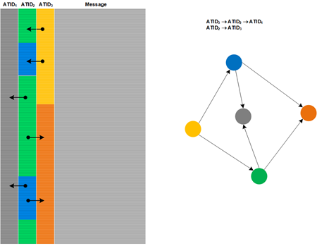
Sometimes, we want to count the number of (Adjoint) Threads of Activity corresponding to a specified ATID:

We can view this as (adjoint) threads coming into or out of the specified ATID, similar to divergence, which gives the name Trace Divergence log analysis pattern. This analysis pattern differs from Cord of Activity, which is not a number, and the latter may not have a single, unvarying source or target ATID to which other A(TID)s correspond. It is also different from Trace Flux, where the number of threads is an external variable not related to traces and logs, and from Message Flow, which operates on the individual message level, temporal in nature, and counters are set in advance.

Typical examples include SYN floods in network traces (src and dst ATIDs), the number of threads corresponding to the specific PID, or the number of threads contending for the specified API.

Activity Divergence may look similar, but its surface is temporal, whereas Trace Divergence’s, surface is structural. There can be several Trace Divergencies in the same trace or log since they are per ATID.

Formally, Trace Divergence is a property of a constructed graph, for example, D_in​(a)=∣{x∈V∣x→a}∣; Activity Divergence is a property of a constructed signal, interpreted as dynamics, for example, D_in​(a,t).

- Dmitry Vostokov @ DumpAnalysis.org + TraceAnalysis.org -

In ARM64 Virtualized Process memory dumps, their Stack Trace Collections, and their Execution Residue we may see pointers that point to ISA-Specific Code. For example, in an x86 process thread stack we may see this x86 disassembly of code pointers:

0:001> u 7573e81c
kernel32!BaseThreadInitThunk+0x2c:
7573e81c 2808 sub byte ptr [eax],cl
7573e81e 0090083142b9 add byte ptr [eax-46BDCEF8h],dl
7573e824 e003 loopne kernel32!BaseThreadInitThunk+0x39 (7573e829)
7573e826 002a add byte ptr [edx],ch
7573e828 0001 add byte ptr [ecx],al
7573e82a 3f aas
7573e82b d6 ???
7573e82c 2808 sub byte ptr [eax],cl

0:001> u 76e12640
KERNELBASE!SetEvent:
76e12640 fd std
76e12641 7bbe jnp KERNELBASE!UnmapViewOfFile+0x11 (76e12601)
76e12643 29fd sub ebp,edi
76e12645 0300 add eax,dword ptr [eax]
76e12647 91 xchg eax,ecx
76e12648 6810009008 push 8900010h
76e1264d a5 movs dword ptr es:[edi],dword ptr [esi]
76e1264e 43 inc ebx

0:001> ub 76e0c11c
^ Unable to find valid previous instruction for 'ub 76e0c11c'

0:001> ub 5f82d9c9
ACE!ACEInitializeEx+0x65573:
5f82d9b7 c3 ret
5f82d9b8 56 push esi
5f82d9b9 57 push edi
5f82d9ba 8b3da8b0835f mov edi,dword ptr [ACE!ACEInitializeEx+0x72c64 (5f83b0a8)]
5f82d9c0 8bf1 mov esi,ecx
5f82d9c2 6aff push 0FFFFFFFFh
5f82d9c4 ff7610 push dword ptr [esi+10h]
5f82d9c7 ffd7 call edi

0:001> ub ntdll!NtWaitForSingleObject+0xc
ntdll!NtMapUserPhysicalPagesScatter:
779fd030 b803000a00 mov eax,0A0003h
779fd035 ba70a6a077 mov edx,offset ntdll!Wow64SystemServiceCall (77a0a670)
779fd03a ffd2 call edx
779fd03c c20c00 ret 0Ch
779fd03f 90 nop
ntdll!NtWaitForSingleObject:
779fd040 b804000d00 mov eax,0D0004h
779fd045 ba70a6a077 mov edx,offset ntdll!Wow64SystemServiceCall (77a0a670)
779fd04a ffd2 call edx

The first 3 look like Wild Code (or Coincidental Symbolic Information if we use function names). But if we switch to CHPE architecture, we get the inverse, the first 3 right and the last 2 invalid:

0:001> .effmach CHPE
Effective machine: CHPE on X86 (read only) (CHPE)

0:001:CHPE> u 7573e81c
kernel32!BaseThreadInitThunk+0x2c:
7573e81c 90000828 adrp x8,kernel32!_imp_#LdrQueryImageFileKeyOption (75842000)
7573e820 b9423108 ldr w8,[x8,#0x230]
7573e824 2a0003e0 mov w0,w0
7573e828 d63f0100 blr x8
7573e82c 90000828 adrp x8,kernel32!_imp_#LdrQueryImageFileKeyOption (75842000)
7573e830 b9429d08 ldr w8,[x8,#0x29C]
7573e834 d63f0100 blr x8
7573e838 36225700 tbz w0,#4,kernel32!#IsFusionFullySupported+0x50 (75743318)

0:001:CHPE> u 76e12640
KERNELBASE!SetEvent:
76e12640 29be7bfd stp wfp,wlr,[sp,#-0x10]!
76e12644 910003fd mov fp,sp
76e12648 90001068 adrp x8,KERNELBASE!__hybrid_auxiliary_iat (7701e000)
76e1264c b943a508 ldr w8,[x8,#0x3A4]
76e12650 2a0003e0 mov w0,w0
76e12654 52800001 mov w1,#0
76e12658 d63f0100 blr x8
76e1265c 37f887e0 tbnz w0,#0x1F,KERNELBASE!BasepCheckImageVersion+0xe8 (76e13758)

0:001:CHPE> ub 76e0c11c
KERNELBASE!#WaitForSingleObjectEx+0xdc:
76e0c0fc 110083a2 add w2,wfp,#0x20
76e0c100 b90017a2 str w2,[fp,#0x14]
76e0c104 53001e61 uxtb w1,w19
76e0c108 2a0203e2 mov w2,w2
76e0c10c 2a0003e0 mov w0,w0
76e0c110 d0001088 adrp x8,KERNELBASE!__hybrid_auxiliary_iat (7701e000)
76e0c114 b9440d08 ldr w8,[x8,#0x40C]
76e0c118 d63f0100 blr x8

0:001:CHPE> ub 5f82d9c9
ACE!ACEInitializeEx+0x65565:
5f82d9a9 000003e8 ???
^ Memory access error in 'ub 5f82d9c9'

0:001:CHPE> ub ntdll!NtWaitForSingleObject+0xc
ntdll!NtAcceptConnectPort+0xc:
779fd02c 900018c2 adrp x2,77d15000
ntdll!NtMapUserPhysicalPagesScatter:
779fd030 0a0003b8 and w24,wfp,w0
779fd034 a670ba00 ???
779fd038 d2ff77a0 mov x0,#-0x443000000000000
779fd03c 90000cc2 adrp x2,77b95000
ntdll!NtWaitForSingleObject:
779fd040 0d0004b8 st1 {v24.b}[1],[x5]
779fd044 a670ba00 ???
779fd048 d2ff77a0 mov x0,#-0x443000000000000

0:001:CHPE> .effmach x86
Effective machine: x86 compatible (x86)

The same is observable for the x64 process thread raw stack region pointers:

0:000> ub 00007ff7`83432ac9
pointers_c!invoke_main+0x16:
00007ff7`83432aa6 4889442430 mov qword ptr [rsp+30h],rax
00007ff7`83432aab e82ae8ffff call pointers_c!ILT+725(__p___argc) (00007ff7`834312da)
00007ff7`83432ab0 8b00 mov eax,dword ptr [rax]
00007ff7`83432ab2 89442420 mov dword ptr [rsp+20h],eax
00007ff7`83432ab6 4c8b442428 mov r8,qword ptr [rsp+28h]
00007ff7`83432abb 488b542430 mov rdx,qword ptr [rsp+30h]
00007ff7`83432ac0 8b4c2420 mov ecx,dword ptr [rsp+20h]
00007ff7`83432ac4 e8b7e7ffff call pointers_c!ILT+635(main) (00007ff7`83431280)

0:000> ub 00007ff8`046917ac
^ Unable to find valid previous instruction for 'ub 00007ff8`046917ac'

0:000> .effmach ARM64EC
Effective machine: ARM64EC (CHPEv2 on X64) (ARM64EC)

0:000:ARM64EC> ub 00007ff7`83432ac9
pointers_c!invoke_main+0x19:
00007ff7`83432aa9 2ae83024 ???
^ Memory access error in 'ub 00007ff7`83432ac9'

0:000:ARM64EC> ub 00007ff8`046917ac
kernel32!$iexit_thunk$cdecl$d$d+0x2c:
00007ff8`0469178c 00000000 ???
kernel32!$iexit_thunk$cdecl$i8$i8:
00007ff8`04691790 d503237f pacibsp
00007ff8`04691794 a9bf7bfd stp fp,lr,[sp,#-0x10]!
00007ff8`04691798 910003fd mov fp,sp
00007ff8`0469179c d10083ff sub sp,sp,#0x20
00007ff8`046917a0 b0000048 adrp x8,kernel32!_os_arm64x_dispatch_call_no_redirect (00007ff8`0469a000)
00007ff8`046917a4 f9400110 ldr xip0,[x8]
00007ff8`046917a8 d63f0200 blr xip0

0:000:ARM64EC> .effmach AMD64
Effective machine: x64 (AMD64)

- Dmitry Vostokov @ DumpAnalysis.org + TraceAnalysis.org -

The Latent Structure pattern addresses situations where a memory region appears raw and untyped yet shows early, incomplete signs of structural organization. Signals, such as small or pointer-like values, alignment regularities, recurring byte sequences, partial strings, or fragments that resemble fields, suggest that a real structure might exist, but cannot yet be interpreted safely or confidently. Latent Structure represents the pre-suspect stage in structural diagnostics: the point where the analyst notices potential form but must resist premature interpretation. Acting too early risks misclassifying problems and misidentifying root causes. Several forces complicate this stage: partial overwrites, coincidental alignments, ABI or version mismatches, and cognitive biases that encourage overinterpretation. This analysis pattern, therefore, emphasizes careful, hypothesis-driven exploration using techniques such as tentative structure casting, pointer-chain heuristics, checks for internal semantic coherence, software internals, and domain knowledge, all without assuming the structure’s validity. When enough evidence accumulates, a Latent Structure transitions into a Suspect Structure (subject of the next analysis pattern), where it becomes testable.

For example, we may see these fragment in Execution Residue:

00000029`e7efeb00 00001f80`0010004b
00000029`e7efeb08 0053002b`002b0033
00000029`e7efeb10 00000242`002b002b

Finally, we write the formal pattern structure card.

Intent

Detect hidden or unclear structural organization in raw memory regions that exhibit early indicators of structure-like form but whose types are not yet known.

Context

Appears in:
Execution Residue, Pointer Cone, Memory Region, and Region Strata.

Problem

A memory dump shows a region of raw bytes without explicit type information that contains hints suggesting that a structure may be present. Prematurely interpreting such memory can lead to false positives, misclassification, incorrect casting, and a chain of misleading hypotheses.

Forces

Data:

• Memory may contain partial structures
• Overwrites blur structure boundaries
• Random-looking regions may hide structured subregions

Semantics:

• Pointer-like values may be real or coincidental
• Partial strings
• Field alignments may appear regular due to chance

Modules:

• Coincidental symbols
• ABI or version mismatches

Cognitive biases:

• Insufficient domain knowledge
• Premature suspicion

Symptoms

• Structural hints in bytes
• Pointer-like values
• Strings and identity hints
• Alignment and regularity
• Recurring patterns across multiple memory locations
• Partial structure validity
• Incomplete or corrupt-like structure

Resolution Strategies

• Structure casting
• Heuristic field and pointer chain analysis
• Verification of internal semantic coherence

Resulting Context

Structure becomes Suspect and testable for validity.

Related Patterns

Hidden Artifact Patterns, Corrupt Structure, Module Hint, Falsity and Coincidence Patterns, Shared Buffer Overwrite, Value References, Small Value, Design Value, Shared Structure, and Regular Data.

Formal Card

- Dmitry Vostokov @ DumpAnalysis.org + TraceAnalysis.org -

When looking at Execution Residue in Windows ARM64 memory dumps, we may notice Encoded Pointers in the form of authenticated pointers (PAC, Pointer Authentication Code, see the Linux guide and Windows info). For example:

0:000> dps 00000053f62fc000 00000053f6300000
...
00000053`f62ffe28 e817fff7`6a0bc054 functions_c!__scrt_common_main+0x14
...

The return address isn’t possible to use directly (Invalid Pointer):

0:000> ub e817fff7`6a0bc054
e817fff7`6a0bc034 ?? ???
^ Memory access error in ‘ub e817fff7`6a0bc054′

However, the symbolic reference is ok:

0:000> ub functions_c!__scrt_common_main+0x14
functions_c!pre_cpp_initialization+0x7c:
00007ff7`6a0bc034 00000000 ???
00007ff7`6a0bc038 00000000 ???
00007ff7`6a0bc03c 00000000 ???
functions_c!__scrt_common_main:
00007ff7`6a0bc040 d503237f pacibsp
00007ff7`6a0bc044 a9bf7bfd stp fp,lr,[sp,#-0x10]!
00007ff7`6a0bc048 910003fd mov fp,sp
00007ff7`6a0bc04c 97ffd81f bl functions_c!ILT+4284(__security_init_cookie) (00007ff7`6a0b20c8)
00007ff7`6a0bc050 94000016 bl functions_c!__scrt_common_main_seh (00007ff7`6a0bc0a8)

Because of that, Rough Stack that uses the dpS WinDbg command instead, omits such valid symbolic references.

If you find such pointers, you can replace the higher 4-byte part with the higher part of the module start address, for example:

0:000> lm
start end module name
00007ff7`6a0a0000 00007ff7`6a0d0000 functions_c
…

0:000> ub 00007ff7`6a0bc054
functions_c!pre_cpp_initialization+0×7c:
00007ff7`6a0bc034 00000000 ???
00007ff7`6a0bc038 00000000 ???
00007ff7`6a0bc03c 00000000 ???
functions_c!__scrt_common_main:
00007ff7`6a0bc040 d503237f pacibsp
00007ff7`6a0bc044 a9bf7bfd stp fp,lr,[sp,#-0×10]!
00007ff7`6a0bc048 910003fd mov fp,sp
00007ff7`6a0bc04c 97ffd81f bl functions_c!ILT+4284(__security_init_cookie) (00007ff7`6a0b20c8)
00007ff7`6a0bc050 94000016 bl functions_c!__scrt_common_main_seh (00007ff7`6a0bc0a8)

Of course, this may not work for pointers, encoded by the Windows EncodePointer API.

Finally, we write the formal pattern structure card for Encoded Pointer.

Intent

To recognize situations where a pointer stored in memory is not directly usable: its value must be interpreted or transformed before it can be resolved to a valid code or data address.

Context

Appears in:
Stack Trace, Execution Residue, Context Pointer, Historical Information.

Common environments:

• Tagged pointers
• ARM64 pointer authentication (PAC)
• Top-Byte-Ignore tagging (AArch64)
• ASLR and relocations that have not yet been applied in the captured memory
• Managed space compressed and metadata-embedded GC pointers
• Objective-C and Swift tagged ISA pointers
• Sanitizers or checking runtimes that add metadata bits

Problem

A pointer in the dump visually appears to be an address, but fails to resolve using normal symbolic or spatial checks; dereferencing its raw value yields an incorrect memory address or a memory error.

Forces

• Performance/security constraints favor encoded pointer formats
• Debugger views often show raw stack/heap
• Encoding schemes vary by platform and compiler
• Hardware PAC may prevent guessing the correct pointer form without a proper decode context

Symptoms

• Pointer value not inside any loaded module or valid virtual address range
• Symbol resolution differs
• Adjacent stack slots look pointer-like, but this one does not
• Backwards disassembly shows an incorrect frame

Resolution Strategies

• Decode PAC
• Canonicalize upper bits
• Strip tags
• Expand bits
• Apply relocation deltas
• Mask metadata

Resulting Context

After correct interpretation, the pointer becomes:

• Resolvable to a target symbol
• Walkable for call-stack reconstruction
• Safe for dereferencing in analysis context
• Enables further analysis

Formal card

- Dmitry Vostokov @ DumpAnalysis.org + TraceAnalysis.org -

The list of local variables displayed by the dv WinDbg command may contain False Local Addresses, especially if some non-standard alignment is used on ARM64 platforms. For example, we get this address that doesn’t look correct if we associate it with the source code:

* _Alignas(4096) long long ll = 1;

0:000> dv /V
0000000b`970fe260 @x27+0×1000 ll = 0n-3689348814741910324
0000000b`970fd490 @x27+0×0230 align = 8

It is not aligned on the page boundary, and the value is not the expected 1:

0:000> dq 0000000b`970fe260 L1
0000000b`970fe260 cccccccc`cccccccc

However, in the disassembly, we see the following sequence of instructions to initialize the variable:

00007ff7`d061afdc f9533f69 ldr x9,[x27,#0x2678]
00007ff7`d061afe0 d2800028 mov x8,#1
00007ff7`d061afe4 f9000128 str x8,[x9]

So, we can see that the local variable address is stored at x27+0×2678:

0:000> dp x27+0x2678 L1
0000000b`970ff8d8 0000000b`970fd000

and see the correct variable value:

0:000> dpp x27+0x2678 L1
0000000b`970ff8d8 0000000b`970fd000 00000000`00000001

This analysis pattern differs from False Effective Address analysis pattern in the correct value of the base register.

- Dmitry Vostokov @ DumpAnalysis.org + TraceAnalysis.org -

On Windows 11 ARM64, it is possible to run x64 and x86 programs (ARM64EC and Compiled Hybrid Portable Executable, CHPE). When we capture memory dumps and examine the corresponding Stack Trace Collection, we see ARM64EC and CHPE frames. This is similar to our earlier Virtualized Process (WOW64) analysis pattern, although WinDbg can show us different architecture frames at the same time. Below are 2 examples of NULL Pointer (Data) analysis pattern.

* x64 process minidump

0:000> ~*kL

. 0 Id: 8030.677c Suspend: 0 Teb: 000000e0`5d015000 Unfrozen
# Arch Child-SP RetAddr Call Site
00 ARM64EC 000000e0`5d2fdf30 00007ff8`02901d6c ntdll!#NtWaitForMultipleObjects+0x14
01 ARM64EC 000000e0`5d2fdf40 00007ff8`046735e0 KERNELBASE!#WaitForMultipleObjectsEx+0xfc
02 ARM64EC 000000e0`5d2fe220 00007ff8`046730e0 kernel32!#WerpReportFaultInternal+0x4c0
03 ARM64EC 000000e0`5d2fe390 00007ff8`0463d3e4 kernel32!#WerpReportFault+0xe0
04 ARM64EC 000000e0`5d2fe3f0 00007ff8`02a047e8 kernel32!#BasepReportFault+0x24
05 ARM64EC 000000e0`5d2fe410 00007ff8`0754f7c4 KERNELBASE!#UnhandledExceptionFilter+0x308
06 ARM64EC 000000e0`5d2fe500 00007ff8`07547148 ntdll!RtlUserThreadStart$filt$0+0x64
07 ARM64EC 000000e0`5d2fe510 00007ff8`0749a304 ntdll!#__C_ExecuteExceptionFilter+0x38
08 ARM64EC 000000e0`5d2fe570 00007ff8`07547068 ntdll!#__C_specific_handler+0xf4
09 ARM64EC 000000e0`5d2fe5f0 00007ff8`07440820 ntdll!#RtlpExecuteHandlerForException+0x28
0a ARM64EC 000000e0`5d2fe610 00007ff8`07546e50 ntdll!#RtlDispatchException+0x298
0b ARM64EC 000000e0`5d2fed90 00007ff7`128d1ccc ntdll!KiUserExceptionDispatcher_DetourReturn+0x10
0c AMD64 000000e0`5d2ff8e0 00007ff7`128d2ac9 pointers_c!main+0x41c
0d AMD64 000000e0`5d2ffdb0 00007ff7`128d2972 pointers_c!invoke_main+0x39
0e AMD64 000000e0`5d2ffe00 00007ff7`128d282e pointers_c!__scrt_common_main_seh+0x132
0f AMD64 000000e0`5d2ffe70 00007ff7`128d2b5e pointers_c!__scrt_common_main+0xe
10 AMD64 000000e0`5d2ffea0 00007ff8`046917ac pointers_c!mainCRTStartup+0xe
11 ARM64EC 000000e0`5d2ffed0 00007ff8`046115e8 kernel32!$iexit_thunk$cdecl$i8$i8+0x1c
12 ARM64EC 000000e0`5d2fff00 00007ff8`0748c120 kernel32!#BaseThreadInitThunk+0x48
13 ARM64EC 000000e0`5d2fff10 00000000`00000000 ntdll!#RtlUserThreadStart+0x70

1 Id: 8030.7a64 Suspend: 0 Teb: 000000e0`5d017000 Unfrozen
# Arch Child-SP RetAddr Call Site
00 ARM64EC 000000e0`5d3ff820 00007ff8`07470084 ntdll!#NtWaitForWorkViaWorkerFactory+0x14
01 ARM64EC 000000e0`5d3ff830 00007ff8`046115e8 ntdll!#TppWorkerThread+0x5a4
02 ARM64EC 000000e0`5d3ffaf0 00007ff8`0748c120 kernel32!#BaseThreadInitThunk+0x48
03 ARM64EC 000000e0`5d3ffb00 00000000`00000000 ntdll!#RtlUserThreadStart+0x70

2 Id: 8030.119c Suspend: 0 Teb: 000000e0`5d019000 Unfrozen
# Arch Child-SP RetAddr Call Site
00 ARM64EC 000000e0`5d4ff980 00007ff8`07470084 ntdll!#NtWaitForWorkViaWorkerFactory+0x14
01 ARM64EC 000000e0`5d4ff990 00007ff8`046115e8 ntdll!#TppWorkerThread+0x5a4
02 ARM64EC 000000e0`5d4ffc50 00007ff8`0748c120 kernel32!#BaseThreadInitThunk+0x48
03 ARM64EC 000000e0`5d4ffc60 00000000`00000000 ntdll!#RtlUserThreadStart+0x70

3 Id: 8030.70f0 Suspend: 0 Teb: 000000e0`5d01b000 Unfrozen
# Arch Child-SP RetAddr Call Site
00 ARM64EC 000000e0`5d5ff810 00007ff8`07470084 ntdll!#NtWaitForWorkViaWorkerFactory+0x14
01 ARM64EC 000000e0`5d5ff820 00007ff8`046115e8 ntdll!#TppWorkerThread+0x5a4
02 ARM64EC 000000e0`5d5ffae0 00007ff8`0748c120 kernel32!#BaseThreadInitThunk+0x48
03 ARM64EC 000000e0`5d5ffaf0 00000000`00000000 ntdll!#RtlUserThreadStart+0x70

4 Id: 8030.4720 Suspend: 0 Teb: 000000e0`5d01d000 Unfrozen
# Arch Child-SP RetAddr Call Site
00 ARM64EC 000000e0`5d6ff740 00007ff8`0487ec00 ntdll!#NtWaitForSingleObject+0x14
01 ARM64EC 000000e0`5d6ff750 00007ff8`0487e2b0 xtajit64!BeginSimulation+0x12eb0
02 ARM64EC 000000e0`5d6ff7a0 00007ff8`0748c0f0 xtajit64!BeginSimulation+0x12560
03 ARM64EC 000000e0`5d6ff7d0 00000000`00000000 ntdll!#RtlUserThreadStart+0x40

0:000> .frame /c 4
04 000000e0`5d2fe3f0 00007ff8`02a047e8 kernel32!#BasepReportFault+0x24
x0=0000000000000003 x1=000000e05d2fe2e0 x2=0000000000000001 x3=0000000000000000
x4=0000000000000000 x5=0000000000000000 x6=0000000000000000 x7=0000000000000000
x8=000000000000012c x9=0000000000000000 x10=0000000000000000 x11=0000000000000000
x12=0000000000000000 x13=0000000000000000 x14=0000000000000000 x15=0000000000000000
x16=0000bbd3fe198401 x17=0000bbd3fe198401 x18=0000000000000000 x19=000000e05d2fe5a0
x20=0000000000000000 x21=000000e05d2fe5a0 x22=00007ff8045a0000 x23=0000000000000000
x24=0000000000000000 x25=0000000000000000 x26=000000e05d2fe410 x27=0000000000000001
x28=0000000000000000 fp=000000e05d2fe3f0 lr=00007ff80463d3e4 sp=000000e05d2fe3f0
pc=00007ff80463d3e4 psr=60000000 -ZC- EL0
kernel32!#BasepReportFault+0x24:
00007ff8`0463d3e4 14000002 b kernel32!#BasepReportFault+0x2c (00007ff8`0463d3ec)

0:000:ARM64EC> .frame /c c
0c 000000e0`5d2ff8e0 00007ff7`128d2ac9 pointers_c!main+0x41c [C:\ACPPWD\pointers_c\pointers_c.c @ 133]
rax=0000000000000004 rbx=0000000000000000 rcx=9ff2ebf5ac870000
rdx=00007ff7128dabc0 rsi=0000000000000000 rdi=000000e05d2ffc18
rip=00007ff7128d1ccc rsp=000000e05d2ff8e0 rbp=000000e05d2ff930
r8=00000000fffffffe r9=0000000000000000 r10=0000000000000001
r11=0000000000000000 r12=0000000000000000 r13=0000000000000000
r14=0000000000000000 r15=0000000000000000
iopl=3 nv up ei pl zr na pe nc
cs=0033 ss=002b ds=002b es=002b fs=0053 gs=002b efl=00003240
pointers_c!main+0x41c:
00007ff7`128d1ccc c70000000000 mov dword ptr [rax],0 ds:00000000`00000004=????????

0:000> .cxr
Resetting default scope

0:000:ARM64EC>

* x86 process full dump

0:000> ~*kL

. 0 Id: 1a68.8a54 Suspend: 0 Teb: 0295d000 Unfrozen
# Arch ChildEBP RetAddr
WARNING: Frame IP not in any known module. Following frames may be wrong.
00 x86 02afe454 779dd5dc 0x2730002
01 x86 02afe458 75eb2f10 ntdll!NtWaitForMultipleObjects+0xc
02 CHPE 02afe460 75eb2f10 KERNELBASE!$push_thunk$stdcall$u$uuuuu+0x60
03 CHPE 02afe4e0 75d30840 KERNELBASE!#WaitForMultipleObjectsEx+0x194
04 CHPE 02afe680 7712bc70 KERNELBASE!#WaitForMultipleObjects+0x20
05 CHPE 02afe690 7712b690 kernel32!#WerpReportFaultInternal+0x598
06 CHPE 02afe790 770e7fe4 kernel32!#WerpReportFault+0x118
07 CHPE 02afe800 75e90da8 kernel32!#BasepReportFault+0x24
08 CHPE 02afe820 779141b4 KERNELBASE!#UnhandledExceptionFilter+0x378
09 CHPE 02afe8f0 77910ef8 ntdll!strrchr+0x1eb4
0a CHPE 02afe910 778cf388 ntdll!#__C_ExecuteExceptionFilter+0x38
0b CHPE 02afe970 77861554 ntdll!#__C_specific_handler+0xf8
0c CHPE 02afe9e0 779b7154 ntdll!RtlpExecuteHandlerForExceptionCHPE+0x14
0d x86 02afeee0 779b7154 ntdll!RtlDispatchExceptionCHPE+0x2de
0e x86 02aff2bc 779e08d2 ntdll!RtlpProcessPushThunkForException+0x7b
0f x86 02aff354 779e0e5f ntdll!RtlDispatchException+0×1ee
10 x86 02aff360 02aff36c ntdll!KiUserExceptionDispatcher+0xf
11 x86 02aff88c 00712a03 0×2aff36c
12 x86 02aff8ac 0071284a pointers_c!invoke_main+0×33
13 x86 02aff908 007126dd pointers_c!__scrt_common_main_seh+0×15a
14 x86 02aff910 00712a88 pointers_c!__scrt_common_main+0xd
15 x86 02aff918 771487a8 pointers_c!mainCRTStartup+0×8
16 CHPE 02aff920 771487a8 kernel32!$push_thunk$cdecl$u$u+0×58
17 CHPE 02aff990 778bfc8c kernel32!BaseThreadInitThunk+0×2c
18 CHPE 02aff9a0 778bfbe8 ntdll!#__RtlUserThreadStart+0×3c
19 CHPE 02aff9f0 7799988c ntdll!#_RtlUserThreadStart+0×28

1 Id: 1a68.8194 Suspend: 0 Teb: 02961000 Unfrozen
# Arch ChildEBP RetAddr
WARNING: Frame IP not in any known module. Following frames may be wrong.
00 x86 086ff5a4 779dee8c 0x2730002
01 x86 086ff5a8 779ab648 ntdll!NtWaitForWorkViaWorkerFactory+0xc
02 CHPE 086ff5b0 779ab648 ntdll!#NtWaitForWorkViaWorkerFactory$push_thunk+0x68
03 CHPE 086ff630 7709e81c ntdll!#TppWorkerThread+0x238
04 CHPE 086ff810 778bfc8c kernel32!BaseThreadInitThunk+0x2c
05 CHPE 086ff820 778bfbe8 ntdll!#__RtlUserThreadStart+0x3c
06 CHPE 086ff870 7799988c ntdll!#_RtlUserThreadStart+0x28

2 Id: 1a68.499c Suspend: 0 Teb: 02965000 Unfrozen
# Arch ChildEBP RetAddr
WARNING: Frame IP not in any known module. Following frames may be wrong.
00 x86 087ffcc4 779dee8c 0x2730002
01 x86 087ffcc8 779ab648 ntdll!NtWaitForWorkViaWorkerFactory+0xc
02 CHPE 087ffcd0 779ab648 ntdll!#NtWaitForWorkViaWorkerFactory$push_thunk+0x68
03 CHPE 087ffd50 7709e81c ntdll!#TppWorkerThread+0x238
04 CHPE 087fff30 778bfc8c kernel32!BaseThreadInitThunk+0x2c
05 CHPE 087fff40 778bfbe8 ntdll!#__RtlUserThreadStart+0x3c
06 CHPE 087fff90 7799988c ntdll!#_RtlUserThreadStart+0x28

3 Id: 1a68.63f4 Suspend: 0 Teb: 02969000 Unfrozen
# Arch ChildEBP RetAddr
WARNING: Frame IP not in any known module. Following frames may be wrong.
00 x86 08b5f854 779dee8c 0x2730002
01 x86 08b5f858 779ab648 ntdll!NtWaitForWorkViaWorkerFactory+0xc
02 CHPE 08b5f860 779ab648 ntdll!#NtWaitForWorkViaWorkerFactory$push_thunk+0x68
03 CHPE 08b5f8e0 7709e81c ntdll!#TppWorkerThread+0x238
04 CHPE 08b5fac0 778bfc8c kernel32!BaseThreadInitThunk+0x2c
05 CHPE 08b5fad0 778bfbe8 ntdll!#__RtlUserThreadStart+0x3c
06 CHPE 08b5fb20 7799988c ntdll!#_RtlUserThreadStart+0x28

0:000> r
eax=001d005b ebx=00000180 ecx=00000003 edx=779ea670 esi=00000000 edi=00000003
eip=02730002 esp=02afe458 ebp=02afe480 iopl=0 nv up ei ng nz ac po cy
cs=001b ss=0023 ds=0023 es=0023 fs=003b gs=0023 efl=00000293
02730002 c3 ret

0:000> .frame /c 7
07 02afe800 75e90da8 kernel32!#BasepReportFault+0x24
x0=0000000000000000 x1=0000000000000000 x2=0000000000000000 x3=0000000000000000
x4=0000000000000000 x5=0000000000000000 x6=0000000000000000 x7=0000000000000000
x8=0000000000000000 x9=0000000000000000 x10=0000000000000000 x11=0000000000000000
x12=0000000000000000 x13=0000000000000000 x14=0000000000000000 x15=0000000000000000
x16=0000000000000000 x17=0000000000000000 x18=0000000000000000 x19=0000000002afe990
x20=0000000002afe990 x21=0000000077090000 x22=0000000000000004 x23=0000000000000000
x24=0000000000000001 x25=0000000075f1e000 x26=0000000000000000 x27=0000000002afe830
x28=0000000002affa38 fp=0000000002afe800 lr=00000000770e7fe4 sp=0000000002afe800
pc=00000000770e7fe4 psr=00000000 ---- EL0
kernel32!#BasepReportFault+0x24:
770e7fe4 2a0003e0 mov w0,w0

0:000:CHPE> .cxr
Resetting default scope

0:000> dps 02aff354
02aff354 02aff88c
02aff358 779e0e5f ntdll!KiUserExceptionDispatcher+0xf
02aff35c 02aff36c
02aff360 02aff3bc
02aff364 02aff36c
02aff368 02aff3bc
02aff36c c0000005
02aff370 00000000
02aff374 00000000
02aff378 00711c6a pointers_c!main+0×3da
02aff37c 00000002
02aff380 00000001
02aff384 00000004
02aff388 00000000
02aff38c 00000000
02aff390 00000000
02aff394 00000000
02aff398 00000000
02aff39c 00000000
02aff3a0 00000000
02aff3a4 00000000
02aff3a8 00000000
02aff3ac 00000000
02aff3b0 00000000
02aff3b4 00000000
02aff3b8 00000000
02aff3bc 0001003f
02aff3c0 00000000
02aff3c4 00000000
02aff3c8 00000000
02aff3cc 00000000
02aff3d0 ffff0ff0

0:000> .cxr 02aff3bc
eax=00000004 ebx=0295a000 ecx=02aff4a0 edx=00000000 esi=02aff6a8 edi=02aff88c
eip=00711c6a esp=02aff6a8 ebp=02aff88c iopl=0 nv up ei pl nz ac po nc
cs=001b ss=0023 ds=0023 es=0023 fs=003b gs=0023 efl=00010212
pointers_c!main+0×3da:
00711c6a c70000000000 mov dword ptr [eax],0 ds:0023:00000004=????????

0:000> kL
*** Stack trace for last set context - .thread/.cxr resets it
# Arch ChildEBP RetAddr
00 x86 02aff88c 00712a03 pointers_c!main+0x3da
01 x86 02aff8ac 0071284a pointers_c!invoke_main+0x33
02 x86 02aff908 007126dd pointers_c!__scrt_common_main_seh+0x15a
03 x86 02aff910 00712a88 pointers_c!__scrt_common_main+0xd
04 x86 02aff918 771487a8 pointers_c!mainCRTStartup+0x8
05 CHPE 02aff920 771487a8 kernel32!$push_thunk$cdecl$u$u+0x58
06 CHPE 02aff990 778bfc8c kernel32!BaseThreadInitThunk+0x2c
07 CHPE 02aff9a0 778bfbe8 ntdll!#__RtlUserThreadStart+0x3c
08 CHPE 02aff9f0 7799988c ntdll!#_RtlUserThreadStart+0x28

- Dmitry Vostokov @ DumpAnalysis.org + TraceAnalysis.org -

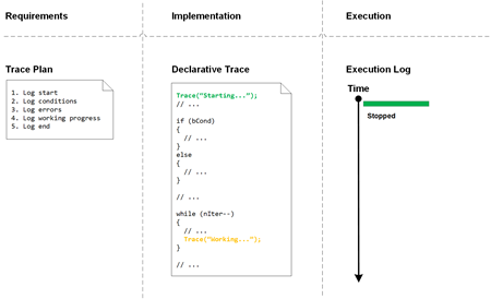
We write software based on requirements and then see its execution. The same analogy can be applied to Declarative Traces, which are “executed.” Trace Plans serve the role of tracing and logging requirements. The following diagram illustrates trace engineering and the lifecycle of tracing and logging:

We look at a resulting trace or log and relate it to its Trace Plan to find anomalies and problems not only in software execution but also in traces and logs themselves and improve tracing source code.

- Dmitry Vostokov @ DumpAnalysis.org + TraceAnalysis.org -

When we get traces and logs, we are interested in Trace Context: an issue description, how its trace was collected, overall system information, related Adjoint Spaces, Trace Summary, and previous traces and logs and their analyses. This contextual information can be organized as a checklist to ensure situational awareness, diagnostic quality, and reduce the number of information request roundtrips.

- Dmitry Vostokov @ DumpAnalysis.org + TraceAnalysis.org -

When we get memory dumps, we are interested in Dump Context: an issue description, how its memory dump was collected, overall system information, related Paratext, and previous memory dumps and their analyses. This contextual information can be organized as a checklist to ensure situational awareness, diagnostic quality, and reduce the number of information request roundtrips.

- Dmitry Vostokov @ DumpAnalysis.org + TraceAnalysis.org -