Software Diagnostics Library

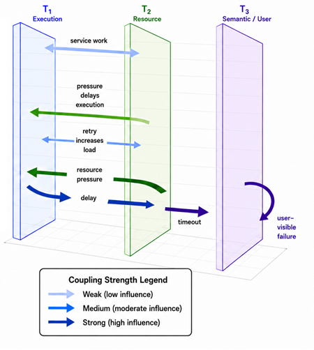
The Trace Multiphysics analysis pattern applies several Trace Fields to the same sequence of trace messages and studies both their individual strengths and their interactions. A Trace Field associates every message in a trace domain M with a value in some analytical range T. Although the field is defined over M, its values need not be extracted solely from that trace. A value may be derived from the message itself, inferred from its surrounding context, or assigned using correlated evidence from other traces, logs, metrics, memory dumps, snapshots, models, or external knowledge sources. The value does not need to be numerical, although numerical or ordered values are useful when field strength must be visualized. For example, one field may represent execution significance, another resource pressure, and a third semantic or user-visible importance:

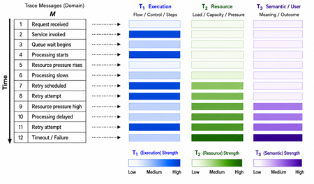
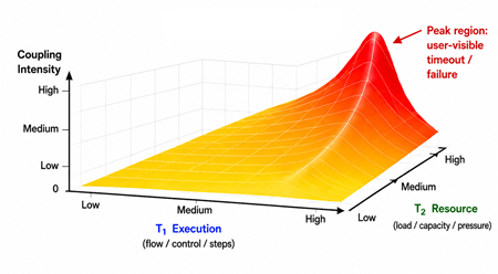
However, Trace Multiphysics is not merely the display of several independent Trace Fields: its essential feature is their coupling. A change in one field may affect another field. For example, increased resource pressure may slow execution. Slower execution may trigger retries. Repeated retries may further increase resource pressure. Eventually, the combined effect may change the semantic or user-visible outcome. The coupling diagram represents these relationships, and arrow thickness indicates coupling strength:

A simple conceptual form is: C_ij​(m)=g(f_i​(m), f_j​(m), R_ij​(m)), where f_i​: M → T_i and f_j​: M → T_j, f_i(m) and f_j(m) are the strengths or values of fields i and j at message m, C_ij(m) is the coupling between fields i and j at message m, and R_ij(m) represents evidence of an interaction between the two fields, obtained from the trace itself or from correlated diagnostic sources. This formula defines coupling at message m. More generally, a coupling may relate field values at different messages when the influence is delayed or propagated through the trace: C_ij​(m_a, m_b)=g(f_i​(m_a), f_j​(m_b), R_ij​(m_a, m_b)), where m_a ⪯ m_b. Here, R_ij​(m_a, m_b) represents evidence relating the value f_i(m_a) of field i to the value f_j(m_b) of field j, whether that evidence is contained in the primary trace or supplied through correlated artifacts. High values in two fields do not automatically establish strong coupling. The available diagnostic evidence must also support the conclusion that one field influences, constrains, amplifies, transforms, or explains the other. Such evidence may occur in the primary trace or in correlated traces, logs, metrics, snapshots, models, or other diagnostic artifacts:

The mapping f_i is defined over the trace domain M, but its construction may depend on evidence outside M. A more explicit form is: f_i(m) = h_i(m, E_i(m)), where E_i(m) is the evidence associated with message m. This evidence may come from the message itself, nearby messages, other traces or logs, metrics, snapshots, memory dumps, learned models, or other correlated diagnostic sources. Correlation may be established through timestamps, identifiers, causal links, shared entities, execution context, or other relations.

When no ordinary field value can be assigned, T_i may include special values representing unknown, unavailable, or not applicable, preserving the definition of the field over the complete trace domain.

In computational modeling, multiphysics simulation studies several aspects of a physical system and their interactions simultaneously. A model may combine thermal, structural, fluid, electromagnetic, or other processes, together with the coupling and boundary conditions between them. Trace Multiphysics transfers this structural principle to software diagnostics. The analogy does not imply that all software behavior should be described by physical equations. Instead, it provides a disciplined way to analyze several interacting dimensions without reducing the incident to one isolated perspective.

The connection is especially appropriate in software diagnostics because software can be its own model. Software execution states and execution artifacts can be copied, preserved, replayed, or analyzed independently. Traces, logs, metrics, memory dumps, and snapshots are symbolic and digital artifacts produced by the software system itself. In this diagnostic sense, software performs a form of self-simulation: its execution generates artifacts that model selected aspects of its own structure and behavior. A trace is not a complete reproduction of the running system. It is a selective, instrumented self-model. Different Trace Fields map messages in that self-model to values in different analytical ranges, each representing a distinct analytical dimension. Some values may be extracted directly from the trace, while others may be inferred, enriched, or projected from correlated traces, logs, metrics, memory dumps, snapshots, models, or external knowledge. Trace Multiphysics studies those fields together and examines how they interact. Thus, multiphysics simulation models several interacting physical processes, whereas Trace Multiphysics analyzes several interacting fields defined over a software-generated model of software behavior and potentially enriched from other diagnostic sources.

Trace Field provides the foundational assignment or mapping from trace messages to values in one analytical range. The field is defined over a selected trace domain, but the evidence used to assign its values may originate inside or outside that domain. Trace Multiphysics extends this principle by applying several Trace Fields to the same trace domain and analyzing their simultaneous values, changing strengths, overlap at individual messages, dependencies, feedback loops, coupling strengths, and combined explanatory effects. The relationship can be summarized as follows: Trace Field maps trace messages to values in one analytical range, while Trace Multiphysics studies several coupled Trace Fields defined over the same trace domain, with their values potentially derived from or enriched by evidence from multiple diagnostic sources.

Trace Multiphysics also connects to several recent analysis patterns. In Trace Reactance, inductive and capacitive effects can be understood as specific forms of inter-field coupling and temporal distortion produced by interacting state fields. Karnaugh Map is also multidimensional but primarily Boolean and combinatorial, whereas Trace Multiphysics accommodates continuous or graded fields, propagation, and feedback loops. Trace World may provide a broader shared diagnostic context in which coupled Trace Fields are interpreted. Bethe Ansatz is a constrained form of Trace Multiphysics in which global behavior is reconstructed from composable pairwise interaction motives.

The pattern is particularly relevant to AI/ML and agentic AI systems. Multiphysics approaches in machine learning usually apply ML to coupled physical processes or incorporate multiple physical priors into learning. Multiphysics-Inspired AI/ML Observability and Diagnostics, by contrast, treats the AI/ML system itself as a collection of interacting analytical fields, including data, optimization, information, computation, uncertainty, control, and semantic outcome fields, defined over a common trace domain constructed from correlated training, inference, and operational events. Its observability aspect concerns the instrumentation, correlation, and enrichment required to construct these fields from training logs, model evaluations, infrastructure metrics, distributed traces, tool-call records, user interactions, safety assessments, and other evidence sources. Its diagnostic aspect concerns how fields interact through their values and couplings, how disturbances propagate across fields, how feedback loops emerge among them, and how their combined effects produce system-level behavior.

In an agentic AI system, for example, increased tool latency may cause retries. Retries may enlarge the accumulated context and increase computational pressure. Context growth may change the relative prominence of relevant information and increase uncertainty, affecting planning, tool selection, and the final semantic outcome. A degraded outcome may provoke further retries, creating a reinforcing feedback loop. Observability provides the correlated evidence needed to construct, expose, and track these fields, while diagnostics analyzes their values and couplings to explain the resulting agent behavior. The behavior cannot be explained adequately by any one field in isolation.

In summary, Trace Multiphysics is a trace and log analysis pattern that examines several Trace Fields defined over the same trace domain, whether their values are derived from that trace alone or assigned using correlated evidence from other diagnostic sources. It studies the immediate, delayed, reinforcing, constraining, transforming, and explanatory couplings through which their combined behavior emerges. Multiphysics-Inspired AI/ML Observability and Diagnostics extends this principle to AI/ML and agentic systems: observability constructs and exposes the relevant fields from distributed evidence, while diagnostics analyzes their interactions and explains the emergent system behavior.

- Dmitry Vostokov @ DumpAnalysis.org + TraceAnalysis.org -

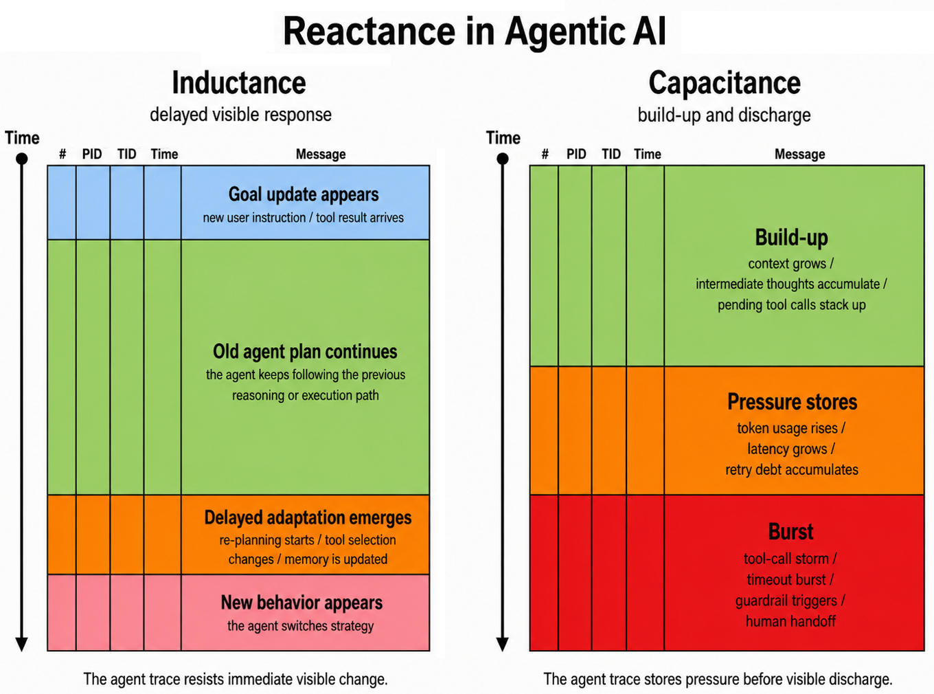
In trace and log analysis, inductance and capacitance can serve as metaphors for two distinct forms of diagnostic behavior.

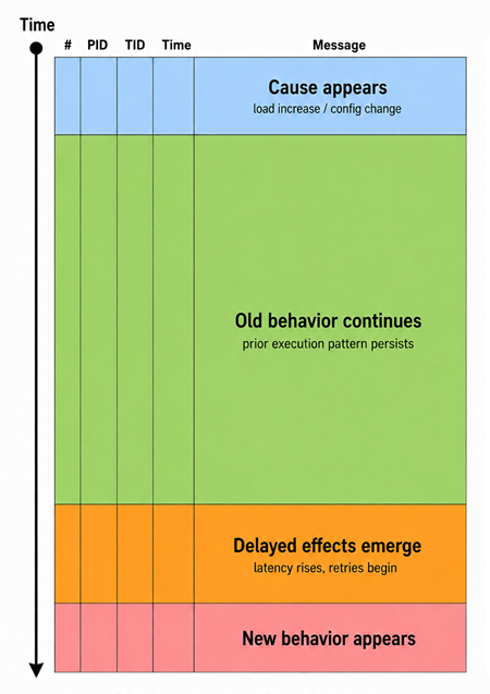
Trace Inductance is the tendency of a system to resist sudden changes in behavior. A new input, configuration change, request burst, or failure condition may not immediately appear in the trace as a new stable pattern. The existing execution flow has “momentum.” Threads, queues, retries, caches, locks, connection pools, batching, and background workers continue to reflect the previous state for some time:

Note that the cause may not be visible in the trace or log but may come from another trace and log, similar to Paratext in memory analysis.

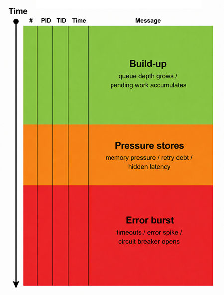
Trace Capacitance is the tendency of a system to accumulate diagnostic potential before a visible discharge occurs. The trace or log may look normal while internal state, queues, memory pressure, retry debt, latency, pending work, or error counters are accumulating. Then the system suddenly emits a burst of Error Messages, warnings, Timeouts, or Phase Transitions.

In summary, Trace Inductance explains delayed behavioral response, and Trace Capacitance explains delayed behavioral manifestation. The former asks: Why did the trace not change immediately after the cause? The latter asks: What was accumulating before the visible failure? Together they help avoid a common mistake: assuming that the first visible error is the real beginning of the problem. In many systems, the cause may appear before the symptom, because of inductance, and the symptom may appear suddenly because of capacitance.

We introduce Trace Reactance as a good umbrella analysis pattern name, with Trace Inductance and Trace Capacitance as two specializations of this pattern: Trace Reactance describes how diagnostic signals are delayed, smoothed, accumulated, or released by the system structure before becoming visible in traces and logs.

An agentic AI fits naturally here, too: agents accumulate context debt, token pressure, and retry state before a sudden degradation in output or a tool-call cascade both inductance and capacitance effects, for example (click on image to enlarge):

- Dmitry Vostokov @ DumpAnalysis.org + TraceAnalysis.org -

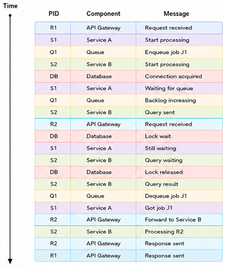
Usually, in traces and logs, messages from different components are highly interleaved. Direct chronological reading may cause confusion because every component’s Adjoint Thread of Activity appears entangled with every other one:

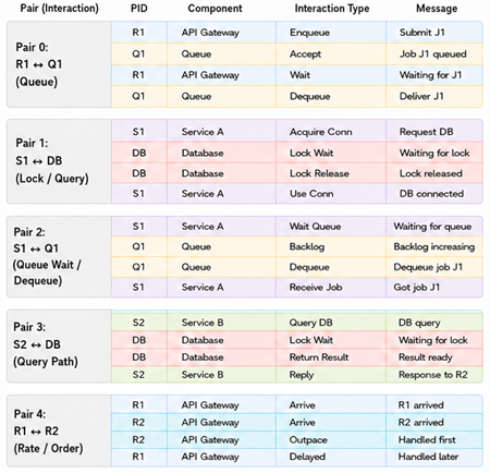
Bethe Ansatz analyzes such a trace by treating requests, threads, agents, transactions, or log-producing entities as “quasi-particles” whose global behavior can be reconstructed from many local pairwise interactions. The inspiration for the pattern name comes from Bethe ansatz, introduced by Hans Bethe in 1931. In physics, it is a method for constructing exact solutions of certain many-body systems: in integrable systems, complex many-body scattering can be represented through factorized two-body scattering processes. In trace analysis, we often face a “many-body” problem: many requests, threads, services, queues, locks, agents, retries, callbacks, and timeouts interact within a single shared diagnostic space. Instead of trying to understand the whole trace as one monolithic event cloud, we decompose it into stable activity lines and pairwise encounters that may explain the global behavior:

The Bethe ansatz has many forms, including coordinate, algebraic, analytic, functional, nested, and thermodynamic variants. For this pattern, the most useful metaphor is the coordinate Bethe ansatz: represent the global state by positions of entities and interaction effects between them. We have the following analogies:

• Particle/excitation: request, thread, transaction, agent, session, workflow
• Coordinate: timestamp, component, hop number, queue position, memory address, trace span
• Momentum/rapidity: (activity) rate, latency class, retry rhythm, priority, causal direction
• Two-body scattering: (pairwise interaction) lock contention, queue wait, API call, resource conflict
• Scattering phase shift: delay, reordered event, changed state, timeout extension, retry offset
• Factorized many-body scattering: whole trace explained as composition of pairwise effects
• Bethe equations: consistency constraints imposed by loops, boundaries, cycles, repeated paths
• Non-integrability: residual behavior not explainable by pairwise interactions

Interactions can be found among Motifs, Macrofunctions, and actors of Activity Theatre.

We suggest the following diagnostic analysis procedure:

1. Identify trace quasi-particles that preserve identity across the trace.
2. Choose a coordinate system: the trace can be read through coordinates other than time.
3. Detect pairwise encounters: look for places where two entities interact; these are diagnostic “scattering” events.
4. Estimate phase shifts where a pairwise encounter often changes the apparent trajectory of an activity. The phase shift is the observable deformation caused by interaction.
5. Test factorization by asking the question: Can the global anomaly be explained as a product of pairwise interactions?

If the answer to the last question is yes, then the system is “Bethe-like”: complex but decomposable. If the answer is no, there may be a true many-body effect, such as shared cache collapse, global scheduler starvation, cascading timeout storm, distributed deadlock, correlated retry amplification, emergent agentic loop, or resource exhaustion caused by collective behavior.

Additionally, we can form a Motivic Trace from the resulting pairwise interaction layers. Motivic Trace compresses a trace into explanatory motives. Bethe Ansatz compresses a trace into pairwise interaction motives whose composition reconstructs the observed global behavior. In this sense, Bethe Ansatz can be viewed as a structured route to Motivic Trace: first decompose the tangled chronological trace into stable activity lines and pairwise encounters; then integrate those encounters into higher-level explanatory motives such as queue delay, database lock wait, retry ordering, and response ordering. In summary: Motivic Trace is the broader compression pattern; Bethe Ansatz is a pairwise-factorized way to build it.

A historical note: this analysis pattern also extends physical analogies of debugging.

- Dmitry Vostokov @ DumpAnalysis.org + TraceAnalysis.org -

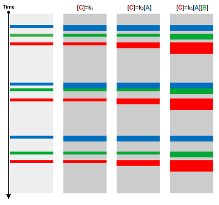
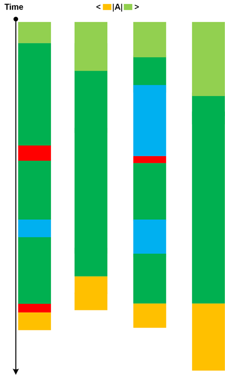
When comparing different traces from the same system we may see different correlations of Statement Densities. For example, when A message density is increased, then C message density is also increased regardless of any changes to B message density. We can borrow concentration notation from chemical kinetics and use [A], [B], and [C] for corresponding Statement Densities, either local in Activity Regions or globally for the whole trace. Observed correlations may point to existing causal mechanisms (like when kinetics points to reaction mechanisms):

This Message Kinetics pattern is more general than Relative Density where a semantic relationship is already known and the comparison is made between working and non-working scenarios. Variations of message densities may occur in normal scenarios, for example, with different amount of input data. There can be several types of Message Kinetics in one trace or log.

- Dmitry Vostokov @ DumpAnalysis.org + TraceAnalysis.org -

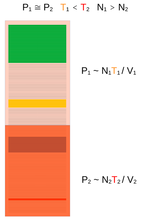
Trace Pressure is a “thermodynamic” variable along with Trace Temperature and Trace Volume. The fourth variable, the number of non-Silent Messages, N, is obvious. In the following diagram, two parts of the trace have approximately the same volume but different “temperature” that result in approx. same “pressure” according to a metaphor of an ideal gas law:

- Dmitry Vostokov @ DumpAnalysis.org + TraceAnalysis.org -

Trace Temperature is an external quantitative (a number) or qualitative (for example, “hot”, “warm”, or “cold”) trace attribute of a trace or log or its fragment such as Activity Region that measures importance of the incident:

It is one example of Trace Field. Being an external attribute, independent from content, the trace with very few or no messages (Sparse Trace) can still have very high “temperature.” However, this analysis pattern is not the same as News Value which is an internal attribute based on trace content that measures its importance.

- Dmitry Vostokov @ DumpAnalysis.org + TraceAnalysis.org -

Trace Volume counts not only messages but also Silent Messages:

The volume metaphor can also be applied to parts of the trace such as Activity Regions, Threads (and Adjoint Threads) of Activity, and various braids.

- Dmitry Vostokov @ DumpAnalysis.org + TraceAnalysis.org -

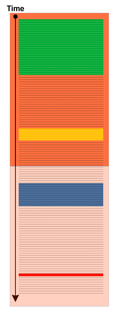
If Trace String analysis patterns caters for trace length variations when the sequence of Activity Regions is constant then Trace Amplitude is about different paths between constant regions at both trace ends that may include varying regions in between, as depicted in the following diagram:

Therefore, several different Trace Strings may be embedded in one Trace Amplitude. The idea of this analysis pattern was borrowed from the path integral formulation of QM.

- Dmitry Vostokov @ DumpAnalysis.org + TraceAnalysis.org -

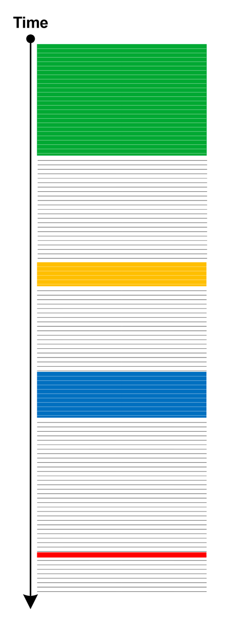
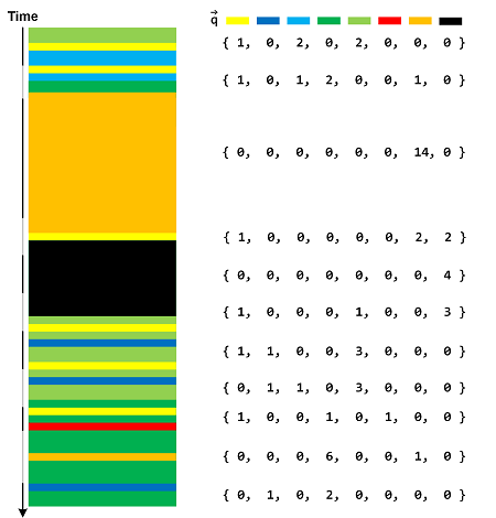
Suppose we are interested in particular message types, which are Message Patterns. We can form a Pattern Vector with values of corresponding Message Pattern occurrences during each fixed time interval corresponding to selected Time Scale. A typical example is illustrated in the following diagram with counted Silent Messages as well:

Each Message Vector component value is the local Statement Current. We can also select Statement Densities instead, especially if we select only Message Patterns from Foreground Components. Other values are possible, for example, from Trace Field.

- Dmitry Vostokov @ DumpAnalysis.org + TraceAnalysis.org -

The relations between Causal History messages (0-chains) can be abstracted as Causal Chains (1-chains). Two relations can be linked if an endpoint of one is also a beginning point of another:

The relations of 1-chains can be abstracted as 2-chains and so on (n-chains):

We took the idea of relation spaces and chains from already quoted “Discreet Causal Theory” book. Causal chain terminology is also used in philosophy.

- Dmitry Vostokov @ DumpAnalysis.org + TraceAnalysis.org -

When looking at Causal History we can choose Causal Messages (not necesseraly the top ones):

Causal Messages may not overlap with the trace Defect Group which may not have any causal relevance being only correlation messages.

- Dmitry Vostokov @ DumpAnalysis.org + TraceAnalysis.org -

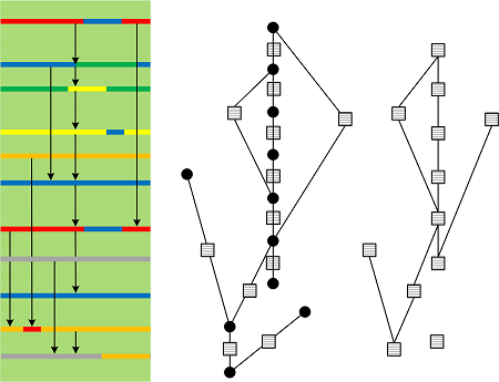
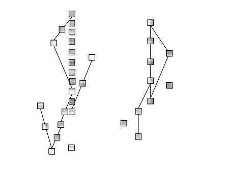
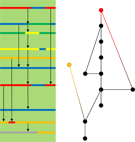
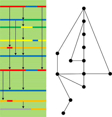
Trace Paths and Back Traces form Causal History of the log where arrows point in the direction of possible causation:

Here we borrow the notion of causal sets from physics and corresponding mathematics. The left diagramming idea was taken from Discrete Causal Theory book and Hasse diagrams (which is inverted in our picture). Also, such graphs are internal to software narratives compared to the more general external space we proposed earlier.

We omit Time arrow as it is possible to consider general traces and logs with their causality markers.

- Dmitry Vostokov @ DumpAnalysis.org + TraceAnalysis.org -

Traces and logs may show drastic qualitative and quantitative pattern changes. We call this analysis pattern Phase Transition by analogy with phase transitions in physical, biological and other complex systems. Usually the goal of the analysis is to find a parameter that caused such transition. Here are a few examples which are self-explanatory.

Change in Statement Density and Current:

Sudden proliferation of (Adjoint) Threads of Activity:

Discontinuity of Activity Region with only Drone Messages left:

- Dmitry Vostokov @ DumpAnalysis.org + TraceAnalysis.org -

Log message “frequencies” in time domain (Statement Current part) are addressed by Fourier Activity analysis pattern. However, we may have varying message density (Statement Density part) across different trace runs (space domain, irrespective of time irregularities):

According to OED, in computing and mathematics a string means “a linear sequence of records or data” and “a sequence of symbols or linguistic elements in a definite order”. So we propose to name this pattern that analyzes densities of messages or Activity Regions as Trace String. Such longitudinal “vibrations” can be compared and analyzed for anomalies across different log runs (Inter-Correlation) or across similar regions in the same log (Intra-Correlation). Here we consider message density change as a one-dimensional displacement. The analogy for this pattern came from one-dimensional vibrating strings (dual resonance model from 1969-70 by Nambu, Nielsen, and Leonard Susskind).

- Dmitry Vostokov @ DumpAnalysis.org + TraceAnalysis.org -

Using the metaphor of renormalization from physics we introduce Renormalization trace and log analysis pattern where a selected message and its Message Context are replaced by a single message:

- Dmitry Vostokov @ DumpAnalysis.org + TraceAnalysis.org -

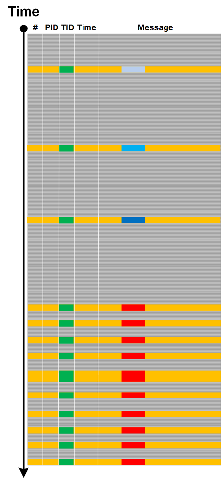
Recently we found a correlation between software trace with high Statement Density and Current of Periodic Error with uniform Error Distribution and process heap Memory Leak suspected from  memory dump analysis. If we metaphorically view periodic errors as “frequency” and the size of a heap as “mass” we may see that the growth of “frequency” correlates with the growth of “mass” and vice versa. Since frequency is inversely proportional to wave length we see a metaphorical analog to Louis de Broglie’s wave-particle duality. In general, as we already pointed in the discussion of narrativity and spatiality of software execution artifacts (see also Software Trace and Memory Dump Analysis seminar), software traces / logs and memory dumps can be seen as “dual” to each other according (metaphorically again) to de Broglie’s “duality of the laws of nature”. So we name this analysis pattern De Broglie Trace Duality since some memory dump regions can be considered of a general trace nature. Our correlation can be depicted in this diagram:

Practically, when we see Memory Consumption Patterns (but don’t know their source / root cause yet) we can ask for traces and logs, and in the case of frequent Periodic Errors found there we can suggest troubleshooting steps that may serve as a resolution or workaround.

- Dmitry Vostokov @ DumpAnalysis.org + TraceAnalysis.org -

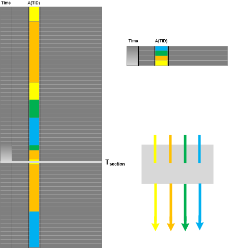
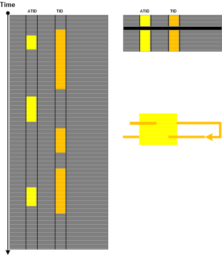
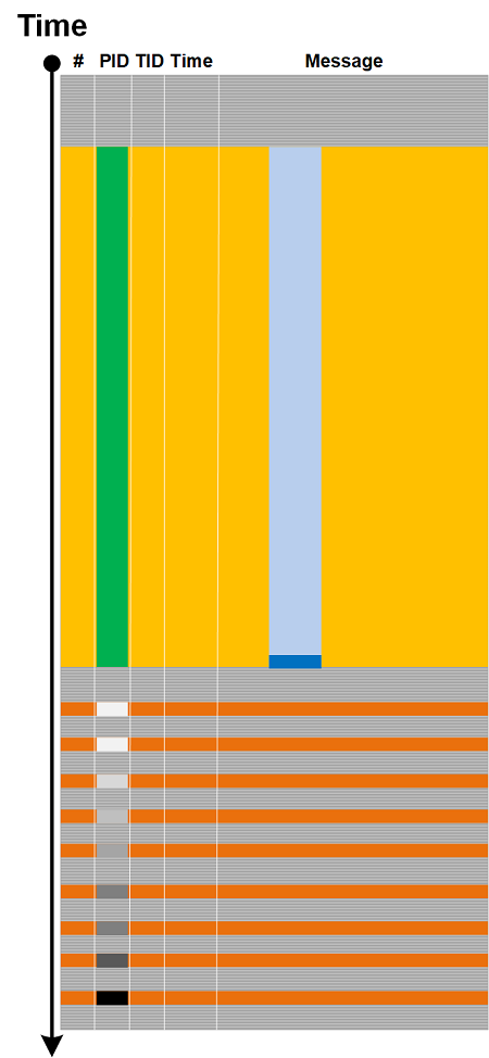
Considering and extending Trace Dimension to TID, ATID, and Time we use Poincaré section and Poincaré map analogies to introduce Poincaré Trace analysis pattern. We choose a value of one “coordinate”, for example, Time, and then form the new trace that consists of messages from different (A)TIDs that have the same timestamp as Time value or the last message(s) from other different ATIDs if they happened before section Time:

If we choose a different ATID than Time and TID, then Poincare Trace is equivalent to Adjoint Thread of Activity. If ATID is TID we have Thread of Activity as a trivial case. If we have Thread of Activity, we can choose some ATID and get Poincaré Trace as illustrated in the following diagram where the thick black line in the right Poincaré Trace represents Discontinuity and its Time Delta:

- Dmitry Vostokov @ DumpAnalysis.org + TraceAnalysis.org -

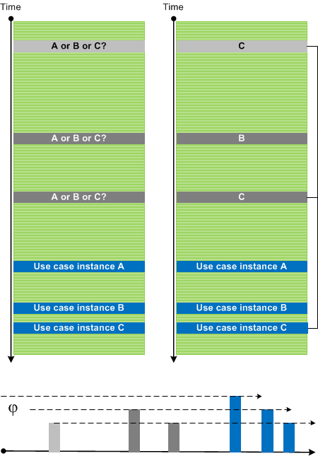
Sometimes we have several use case instances traced in one log file. Messages and Activity Regions from many Use Case Trails intermingle and make analysis difficult especially with the absence of UCID (Use Case ID), any other identification tags, or Message Links. However, initially most of the time we are interested in a sequence of Significant Events. After finding Anchor Messages we can use Time Deltas to differentiate between trace statements from different Use Case Trails. Here we assume correct Event Sequence Order. We call this pattern Event Sequence Phase by analogy with wave phases (all such individual “waves” may have different “shapes” due to various delays between different stages of their use case and implementation narratives):

In the picture above we also identified Dominant Event Sequence for use case instance C.

- Dmitry Vostokov @ DumpAnalysis.org + TraceAnalysis.org -